4 Random effects
In some cases we may have measured variables whose effects we would like to treat as random. Often the distinction between fixed and random is given by example: things like city, species, individual and vial are random, but sex, treatment and age are not. Or the distinction is made using rules of thumb: if there are few factor levels and they are interesting to other people they are fixed. However, this doesn’t really confer any understanding about what it means to treat something as fixed or random, and doesn’t really allow judgements to be made for variables in which the rules of thumb seem to contradict each other. Similarly, these ‘explanations’ don’t give any insight into the fact that all effects are technically random in a Bayesian analysis.
Random effect models are often expressed as an extension of Equation (3.2):
\[E[{\bf y}] = {\bf X}{\boldsymbol{\mathbf{\beta}}}+{\bf Z}{\bf u} \label{MM} \tag{4.1}\]
where \({\bf Z}\) is a design matrix like \({\bf X}\), and \({\bf u}\) is a vector of parameters like \({\boldsymbol{\mathbf{\beta}}}\). However, at this stage there is simply no distinction between fixed and random effects. We could combine the design matrices (\({\bf W} = [{\bf X}, {\bf Z}]\)) and combine the vectors of parameters (\(\boldsymbol{\theta} = [{\boldsymbol{\mathbf{\beta}}}^{'}, {\bf u}^{'}]^{'}\)) to get:
\[E[{\bf y}] = {\bf W}\boldsymbol{\theta} \label{MM2} \tag{4.2}\]
which is identical to Equation (4.1). So if we don’t need to distinguish between fixed and random effects at this stage, when should we distinguish between them, and what distinguishes them?
When we treat an effect as random we believe that the coefficients have some distribution around a mean of zero; often we assume they are normal12 and that they are independent (represented by an identity matrix) and identically distributed with variance \(\sigma^{2}_{u}\):
\[{\bf u} \sim N({\bf 0}, {\bf I}\sigma^{2}_{u})\]
\(\sigma^{2}_{u}\) is a parameter of the model which we estimate, in addition to \({\bf u}\). In a Bayesian analysis we would also assign \(\sigma^{2}_{u}\) a prior, and \(\sigma^{2}_{u}\) is often called a hyper-parameter with an associated hyper-prior.
Fixed effects in a frequentist analysis are not assigned a distribution, but we can understand this in terms of the limit to the normal distribution
\[\boldsymbol{\beta} \sim N({\bf 0}, {\bf I}\sigma^{2}_{\beta})\]
as \(\sigma^{2}_{\beta}\) tends to infinity. In a Bayesian setting we would call this a flat improper prior. In practice, we often use diffuse proper priors in Bayesian analyses. For example, the default in \(\texttt{MCMCglmm}\) is to set \(\sigma^{2}_{\beta}=10^8\). Then, \(\boldsymbol{\beta}\) are technically random - they are assigned a distribution - but I find it useful to retain the frequentist terminology ‘fixed’. The only difference then is that the ‘fixed’ effects are assigned a prior distribution with a variance that is defined by the user-specified prior (\(\sigma^{2}_{\beta}\) - which is often set to be large) and the ‘random’ effects are assigned a prior distribution with a variance that is estimated (\(\sigma^{2}_{u}\) - which could be large, but also zero).
That is the distinction between fixed and random effects. The difference really is that simple, but it takes a long time and a lot of practice to understand what this means in practical terms, and why working with random effects can be a very powerful way of modelling data. To get a feel for why we might want to fit an effect as random or not, lets work through an example before moving on to model fitting. In Section 3.6 we analysed binomial data where 122 respondents had looked at 44 photographs of people and given them a ‘grumpy score’ of more than five (a success) or less than five (a failure). If, instead of 122 respondents, there had been a zillion respondents, we could use the average proportion of success for each photo as a nearly perfect estimates of their probabilities of success. The variance of these near-perfect estimates could serve as a reasonable estimate of the variance in photo effects. If the probabilities were all clustered tightly around 0.5: 0.505, 0.501, 0.499 and so on, then variance would be estimated to be small. Let’s then imagine that we obtained a \(45^\textrm{th}\) photograph but by this point the respondents were so bored I managed to only recruit a single person who gave the photo a score greater than five - a success. Since we only have one observation for this photo the average proportion of success would be one. Do you think the best estimate of the probability of success for the \(45^\textrm{th}\) photograph is then 1.000? I think you wouldn’t: you would use the knowledge that you have gained from the other photos and say that it is more likely that if you had managed to recruit more respondents you would have got a roughly even split of success and failures. You have used common sense, treated the photo effects as random, and shrunk photo 45’s effect towards the average because the variance (\(\sigma^2_u\)) was small and we have a strong prior. If we had treated the photo effects as fixed, we believe that the only information regarding a photo’s value comes from data associated with that particular photo, and the estimate of photo 45’s probability would have been one. When we treat an effect as random, we also use the information that comes from data associated with that particular photo (obviously), but we weight that information by what the data associated with other photos tell us about the likely values that the effect could take - through the parameter \(\sigma^2_u\). What if the probabilities weren’t all clustered tightly around 0.5, but took on values 0.500, 0.998, 0.002, 0.327 …? The variance \(\sigma^2_u\) would be larger and the prior information for our \(45^\textrm{th}\) photo would be weaker: perhaps we got a success because the underlying probability was 0.998, but a single success would also not be very surprising if the underlying probability was 0.500, or even 0.327. We might then be happy that our best estimate of the probability of success for the \(45^\textrm{th}\) photograph was close to one, although with such weak prior information (large \(\sigma^2_u\)) the uncertainty would remain large.
When the motivation for treating an effect as random is explained this way, it is hard to come up with a reason why you wouldn’t treat all effects as random. However, you have to consider how much information is in a given data set to estimate \(\sigma^2_u\), which we will cover in Section 4.9.
4.1 Generalised Linear Mixed Model (GLMM)
In Section 3.6, the binomial model we fitted only contained fixed effects, as specified in the fixed argument to MCMCglmm (fixed=cbind(g5,l5)~type+ypub). No random effects were fitted, although ‘residuals’ were fitted as default to absorb any overdispersion. Residuals are random effects for which we estimate a variance - the hyperparameter, \(\sigma^2_e\) - and when used with Binomial or Poisson responses are commonly referred to as observation-level random effects. Since there is a one-to-one correspondence between observation and photo in this data set, \(\sigma^2_e\) is equivalent to the \(\sigma^2_u\) discussed above (although \(\sigma^2_e\) refers to the variance on the logit scale rather the probability scale used implicitly above). We saw that the probability of success varied greatly across photos (model mbinom.1) but we also noted that some of this variation may be due to the person being photographed and we could tease apart the effect of person from the specifics of the photo since each person was photographed twice - once when happy and once when grumpy. \(\texttt{person}\) has 22 levels and you are probably not interested in knowing the grumpy score of someone you didn’t know - \(\texttt{person}\) effects seem to satisfy the rule of thumb often used to decide that they should be treated as random. The random effect model is specified through the argument random and for simple effects as these we simply put the name of the corresponding column (\(\texttt{person}\)) in the model formula. We will also specify inverse-Wishart priors for both the residual variance and the variance of the \(\texttt{person}\) effects (see Section 2.6) although scaled non-central \(F\)-distribution priors are recommended for random-effect variances (see Section 4.6):
prior.mbinom.2=list(R=list(V=1, nu=0.002), G=list(G1=list(V=1, nu=0.002)))

mbinom.2<-MCMCglmm(cbind(g5, l5)~type+ypub, random=~person, data=Grumpy, family="binomial", pr=TRUE, prior=prior.mbinom.2)
summary(mbinom.2)
##
## Iterations = 3001:12991
## Thinning interval = 10
## Sample size = 1000
##
## DIC: 5376.535
##
## G-structure: ~person
##
## post.mean l-95% CI u-95% CI eff.samp
## person 0.8571 0.008145 1.644 744.3
##
## R-structure: ~units
##
## post.mean l-95% CI u-95% CI eff.samp
## units 0.5662 0.2551 1.03 757.7
##
## Location effects: cbind(g5, l5) ~ type + ypub
##
## post.mean l-95% CI u-95% CI eff.samp pMCMC
## (Intercept) -0.69340 -1.71089 0.32701 1000 0.170
## typehappy -1.28947 -1.73468 -0.80224 1000 <0.001 ***
## ypub 0.01961 -0.01583 0.05956 1000 0.292
## ---
## Signif. codes: 0 '***' 0.001 '**' 0.01 '*' 0.05 '.' 0.1 ' ' 1We can see that the between-person variance is comparable to the residual (across-photo within-person) variance although the credible intervals on both variances is wide. \(\texttt{MCMCglmm}\) does not store the posterior distribution of the random effects by default, as there may be a lot of them and they are often not of interest. However, since I specified pr=TRUE, the whole of \(\boldsymbol{\theta}\) is stored rather than just \({\boldsymbol{\mathbf{\beta}}}\). In Section 3.6 we saw that photo 4521 and photo 4527, despite having the same fixed effect prediction (\(\texttt{type}\) = \(\texttt{grumpy}\), \(\texttt{ypub}\) = 16 years), had quite different probabilities of success, with the posterior mean probabilities being 0.862 and 0.400 respectively. What we didn’t know is whether this divergence in probability was due to the person being photographed or some property of the photo.
4.2 Prediction with Random Effects
If we use the \(\texttt{predict}\) method on our model the default is to not only marginalise the residuals, but also to marginalise any other random effects. If we predict the probability of success for these two photos they are identical, because we are calculating the expectation based on \({\bf X}{\boldsymbol{\beta}}\) only:
##         3        25
## 0.4268878 0.4268878
The \(\texttt{predict}\) method (and \(\texttt{simulate}\) method) for \(\texttt{MCMCglmm}\) includes the argument \(\texttt{marginal}\) which by default takes the \(\texttt{random}\) argument used to fit the model. If we want to obtain a prediction that includes (some of) the random effects we can remove the corresponding term from the formula passed to \(\texttt{marginal}\). Since we only have one random term, which we like to include in the prediction, \(\texttt{marginal}\) is empty:
##          fit       lwr       upr
## 3  0.6305977 0.4239065 0.8337487
## 25 0.3926134 0.2243962 0.5917725
It seems that some of the divergence in probability is due to the person being photographed: our best estimate is that if we had taken many photos of \(\texttt{darren_o}\) when grumpy 63.1 % of people would have scored him above five on the grumpy scale, but for \(\texttt{craig_w}\) it would be lower (39.3 %). The 95% credible (confidence) intervals on each are wide however, and a formal comparison (on the logit scale) gives a 95% credible interval that overlaps zero:
##           lower    upper
## var1 -0.1010677 2.502953
## attr(,"Probability")
## [1] 0.95
4.3 Overdispersed Binomial as a Bernoulli GLMM
The \(\texttt{Grumpy}\) data set aggregates the scores of the 122 respondents into a single binomial response for each photograph. However, we could imagine disaggregating the data such that each respondent for each photograph gets a Bernoulli response with a success if they gave a particular photo a score greater than five. The disaggregated data (FullGrumpy) have \(122\times 44 = 5,368\) observations (although a few respondents did not assess all photos).
##   y   type photo person age ypub respondent student
## 1 9 grumpy  4511 ally_p  38   13          1      NO
## 2 8 grumpy  4511 ally_p  38   13          2      NO
## 3 3 grumpy  4511 ally_p  38   13          3      NO
\(\texttt{y}\) is now the score each respondent \(\texttt{respondent}\) gave each \(\texttt{photo}\) (rather than the average score for each \(\texttt{photo}\) in Grumpy). In addition, we have the respondent-level information \(\texttt{student}\) which can be either \(\texttt{YES}\) or \(\texttt{NO}\). We will turn each persons score into the Bernoulli response
and fit the model
prior.mbinom.3=list(R=list(V=1, fix=1), G=list(G1=list(V=1, nu=0.002), G2=list(V=1, nu=0.002)))

mbinom.3<-MCMCglmm(g5~type+ypub, random=~person+photo, data=FullGrumpy, family="binomial", prior=prior.mbinom.3)

summary(mbinom.3)
##
## Iterations = 3001:12991
## Thinning interval = 10
## Sample size = 1000
##
## DIC: 5332.549
##
## G-structure: ~person
##
## post.mean l-95% CI u-95% CI eff.samp
## person 1.046 0.0005014 2.173 308.1
##
## ~photo
##
## post.mean l-95% CI u-95% CI eff.samp
## photo 0.8689 0.3223 1.717 210.6
##
## R-structure: ~units
##
## post.mean l-95% CI u-95% CI eff.samp
## units 1 1 1 0
##
## Location effects: g5 ~ type + ypub
##
## post.mean l-95% CI u-95% CI eff.samp pMCMC
## (Intercept) -0.84769 -1.97064 0.42422 886.5 0.162
## typehappy -1.49164 -2.13927 -0.94842 749.9 <0.001 ***
## ypub 0.02431 -0.02036 0.06655 1000.0 0.240
## ---
## Signif. codes: 0 '***' 0.001 '**' 0.01 '*' 0.05 '.' 0.1 ' ' 1The random effects deal with any variation in the probability of success across photos and are exactly comparable to the residuals of the binomial model mbinom.2. It is therefore surprising that the posterior distributions for both the variance in \(\texttt{person}\) effects and the variance in \(\texttt{photo}\)/residual effects appear to be different between the two models, as do the fixed effects. This is a peculiarity of logit-link models in \(\texttt{MCMC}\) and wouldn’t be seen in \(\texttt{family="threshold"}\) models that implements the standard probit link. In the binomial model mbinom.2 we implicitly assumed that the probability of success did not vary across respondents within photos - this was an assumption, and one that cannot be tested. In the Bernoulli model mbinom.3 we explicitly assumed that the probability of success varied across respondents within photos, and the variance on the logit-scale was one. Since Bernoulli data provide no information about observation-level variability either (or most likely, neither) assumption could be true but we have no way of knowing (Section 3.6.3). As we saw with fixed effect coefficients in Bernoulli GLM, stating that the variances in photo effects is 0.869 is meaningless in a Bernoulli GLMM without putting it in the context of the assumed residual variance. The standard approach - what I refer to as the standard logit model - is to assume the residual variance is zero. While I think this is a good standard, this is prohibited in \(\texttt{MCMCglmm}\) because the chain will not mix. But as we saw with the fixed effects, we can rescale the variances by needs to be multiplied by \(1/(1+c^{2}\sigma^{2}_{\texttt{units}})\) where \(c=16\sqrt{3}/15\pi\) and \(\sigma^{2}_{\texttt{units}}\) is our assumed residual variance, which is one (Figure 4.1).
c2 <- ((16*sqrt(3))/(15*pi))^2

rescale.VCV.2 <- mbinom.2$VCV
colnames(rescale.VCV.2)[2]<-"photo"

rescale.VCV.3 <- mbinom.3$VCV[,c("person", "photo")]/(1+c2)

plot(mcmc.list(as.mcmc(rescale.VCV.2), as.mcmc(rescale.VCV.3)), density=FALSE)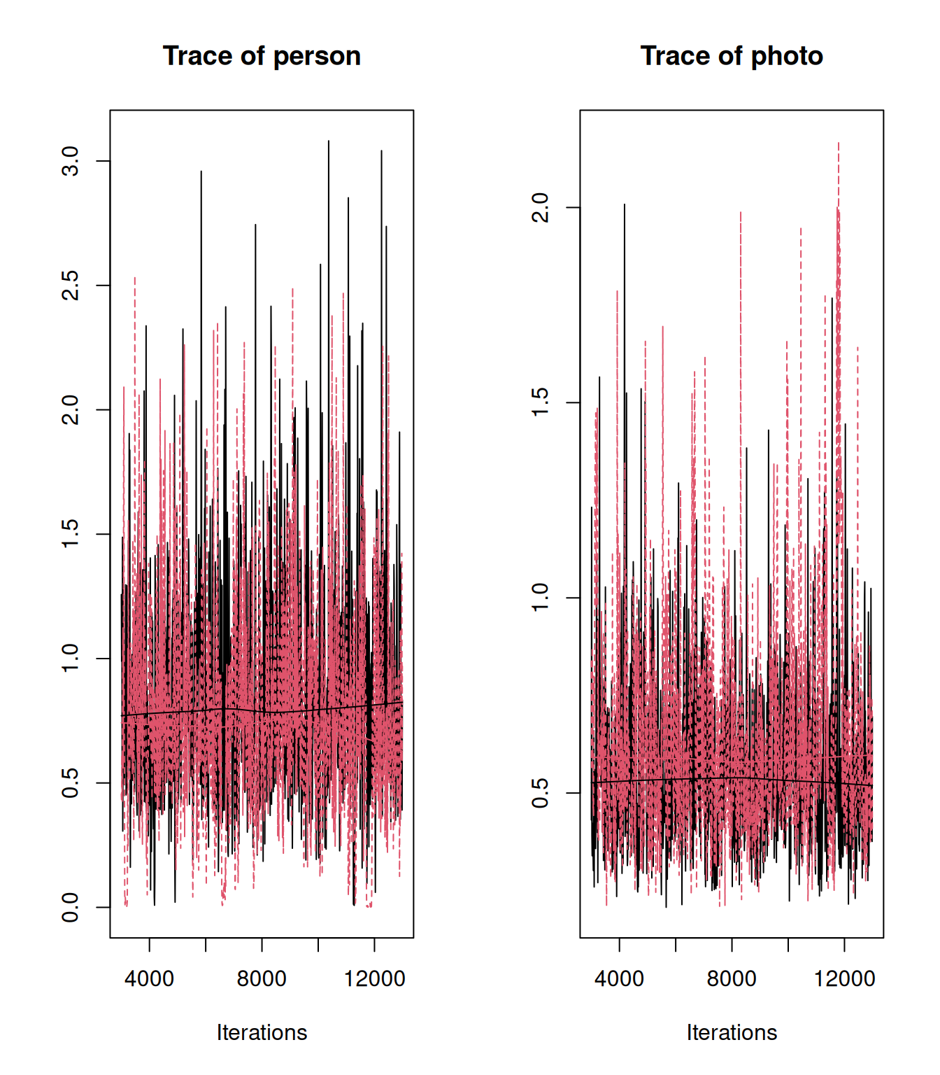
Figure 4.1: MCMC traces for the estimated variances in \(\texttt{person}\) and \(\texttt{photo}\) effects from a Bernoulli GLMM (model mbinom.3) of individual data (red) and a Binomial GLMM (model mbinom.2) where all data for a photo have been aggregated into a single Binomial response (black). The posterior distribution of the variances from the Bernoulli GLMM have been rescaled to what would be observed if the residual variance was zero (rather than one).
4.4 Intra-class Correlations
A more common approach, however, is to express the variances as intra-class correlations where we take the variance of interest and express it as a proportion of the total. For example, for the \(\texttt{person}\) effects, the intra-class correlation would be
\[ICC = \frac{\sigma^2_{\texttt{person}}}{\sigma^2_{\texttt{person}}+\sigma^2_{\texttt{photo}}+\sigma^2_{\texttt{units}}+\pi^2/3}\]
where the \(\pi^2/3\) appears because we have used the logit link and this is the link variance (the variance of the unit logistic).
ICC.2 <- mbinom.2$VCV/(rowSums(mbinom.2$VCV)+pi^2/3)
colnames(ICC.2)[2]<-"photo"

ICC.3 <- mbinom.3$VCV[,c("person", "photo")]/(rowSums(mbinom.3$VCV)+pi^2/3)

plot(mcmc.list(as.mcmc(ICC.2), as.mcmc(ICC.3)), density=FALSE)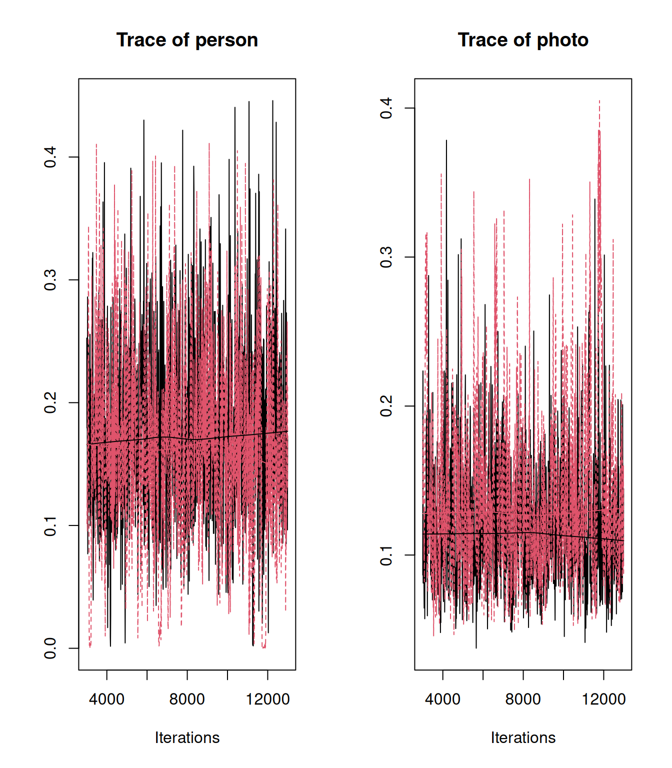
Figure 4.2: MCMC traces for the estimated intra-class correlation for \(\texttt{person}\) and \(\texttt{photo}\) effects from a Bernoulli GLMM (model mbinom.3) of individual data (red) and a Binomial GLMM (model mbinom.2) where all data for a photo have been aggregated into a single Binomial response (black).
If we had used \(\texttt{family="threshold"}\) this would be omitted because the link variance is zero as we are already working on the … scale13 Pierre de Villemereuil’s \(\texttt{QGLMM}\) package.
The eagle-eyed will have noticed that although the trace plots for the rescaled variance/intra-class correlation for the \(\texttt{person}\) effects look identical between the two models, the trace plots for the \(\texttt{photo}\) effects look slightly different with the posterior from model mbinom.3 (the Bernoulli GLMM in red) appearing to have more density at higher values. However, this difference is due to Monte Carlo error, which is quite high for the variance estimates because the autocorrelation in the chain is moderate. The reported effective sample size in the model summary gives some indication of this - for example in the Bernoulli model the effective sample size for the variance in \(\texttt{photo}\) effects is 211, quite a bit less than the 1,000 samples saved (Section 2.5.4). We can see this more clearly if we just plot the traces for Bernoulli model (Figure 4.3).
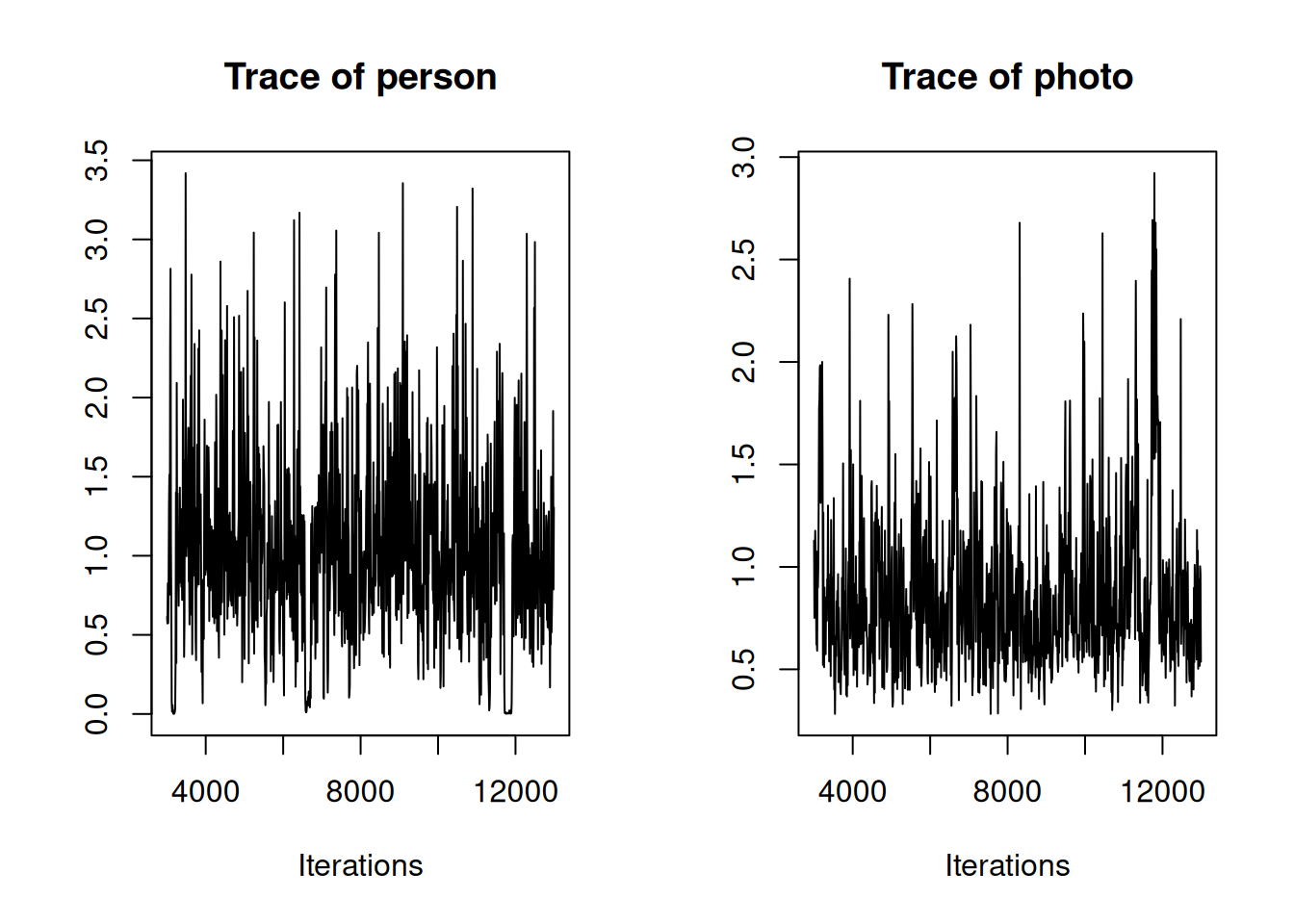
Figure 4.3: MCMC trace for the variances in \(\texttt{person}\) and \(\texttt{photo}\) effects from a Bernoulli GLMM (model mbinom.3).
Two things are apparent from Figure 4.3. Autocorrelation is present - this is not surprising: for each iteration of the MCMC chain the random effects are Gibbs sampled conditional on their variance in the previous iteration, and then conditional on the updated random effects the variances are then Gibbs sampled (Section 2.5). This will invariably lead to autocorrelation. Second, the trace for the variance in \(\texttt{person}\) effects appears to intermittently get ‘stuck’ at values close to zero. In part, this reflects the mechanics of the Gibbs sampling, but it is also a consequence of the inverse-Wishart prior used which has a sharp peak in density at small values (Section 2.6). When the variance in \(\texttt{person}\) effects gets ‘stuck’ at zero, the variance in \(\texttt{photo}\) effects appears to get ‘stuck’ at high values. This is because the data provide strong support for the combined effect of \(\texttt{photo}\) and \(\texttt{person}\) being large, but contain less information about their separate effects. Consequently, if the \(\texttt{person}\) variance drops to zero, the \(\texttt{photo}\) variance increases to compensate. In this example, the effects described above are quite subtle, and simply running the chain for longer would probably suffice. However, a better general strategy would be to employ parameter expansion and use scaled non-central \(F\) priors.
4.5 Underdispersion
Underdispersion in GLMM is likely to create problems. While (G)LMM are parameterised in terms of variances, it is possible - and advisable - to think about them as modelling the covariances between observations belonging to the same group. In the context of the data collected on photos, underdispersion would arise if there were negative covariances in the probability of success between the Bernoulli trials of each photo that we aggregate into the binomial response. Since the variance parameters are really covariance parameters, the best estimate for the units ‘variance’ in the binomial would be negative. However, because GLMM are parameterised in terms of variances, negative values are prohibited and the best estimate would lie on the boundary at zero. This can also impact the estimate of the variances for other random effects - because the total ‘variance’ is negative, positive values of the variances at other levels are disfavoured.
I don’t see this as an issue with GLMM, but an issue with the choice of distribution. The binomial arises from independent trials with a fixed probability. When underdispersion occurs, we are envisaging that the trials are no longer independent. When they were dependent but positively correlated we could accommodate the resulting overdispersion by letting the probability of success vary over photos. When they are dependent but negatively correlated, and therefore underdispersed, we can’t use this trick - the data are simply not binomially distributed and we can’t model our way out of that. Similarly, the Poisson distribution arises as the distribution of the number of events that occur in a fixed amount of time if they appear independently and at constant rate. If events are dependent but positively correlated, we can accommodate this overdisperion by allowing the rate to vary over observations. If events are dependent but negatively correlated we can’t use this trick - the data are simply not Poisson distributed. Family sizes are a good example. You have a kid. You have another kid for them to play with. You’re tired and broke and so stop having kids. Whereas a Poisson process is memoryless, a parent isn’t, and we would need a distribution that allowed for that.
4.6 Priors for Random Effect Variances
Parameter expansion is an algorithmic trick for speeding up the mixing and convergence of the MCMC chain. An unintended but useful side-effect of parameter expansion is that it can allow a wider class of prior distributions while still permitting Gibbs sampling (Chapter 2). In order to explore parameter expansion, and the associated \(F\) prior for random-effect variances, we will work with a model and data-set where the issues noted for model mbinom.3 are much more obvious - the Schools example discussed in Gelman (2006).
schools<-data.frame(school= letters[1:8],
                    estimate= c(28.39, 7.94, -2.75 , 6.82, -0.64, 0.63, 18.01, 12.16),
                    ve = c(14.9, 10.2, 16.3, 11.0, 9.4, 11.4, 10.4, 17.6)^2)
head(schools)
## school estimate ve
## 1 a 28.39 222.01
## 2 b 7.94 104.04
## 3 c -2.75 265.69
## 4 d 6.82 121.00
## 5 e -0.64 88.36
## 6 f 0.63 129.96The response variable estimate is the relative effect of Scholastic Aptitude Test coaching programs in 8 schools and Gelman (2006) focusses on the variance in school effects. Since we only have a single estimate per school there will be a one-to-one mapping between \(\texttt{school}\) effects and the residual. In most cases this would result in the variance in school effects being confounded with the residual variance. Here, however, we have been gifted the residual (within school) variance (\(\texttt{ve}\)) which varies from school to school. In reality, these residual variances are actually estimates and we might wish to factor in this additional complication, but for now we will ignore this complexity and come back to it in Chapter 9. First, lets fit the inverse-Wishart prior we have been using up to now with \(\texttt{V}=1\) and \(\texttt{nu}=0.002\). This prior is equivalent to an inverse-gamma prior with a shape and scale of 0.001 (Section 2.6):
prior.mschool.1<-list(R=list(V=diag(schools$ve), fix=1),
                      G=list(G1=list(V=1, nu=0.002)))

mschool.1<-MCMCglmm(estimate~1, random=~school, rcov=~idh(school):units, data=schools, prior=prior.mschool.1)
The model contains an argument we haven’t seen before: \(\texttt{rcov}\). In all previous analyses we used the default ~units which fits a set of independent and identically distributed residuals with a single variance (\(\sigma^2_{\texttt{units}}\)) to be estimated. \(\texttt{MCMCglmm}\) allows this assumption to be relaxed, and Chapter 5 is dedicated to this subject. Here, we will simply note that we have assigned each school a residual variance (the corresponding element of \(\texttt{ve}\)) and fixed it at this value, leaving only the intercept and the variance in school effects (\(\sigma^2_{\texttt{school}}\)) to be estimated. The MCMC trace for \(\sigma^2_{\texttt{school}}\) looks dreadful (Figure 4.4).
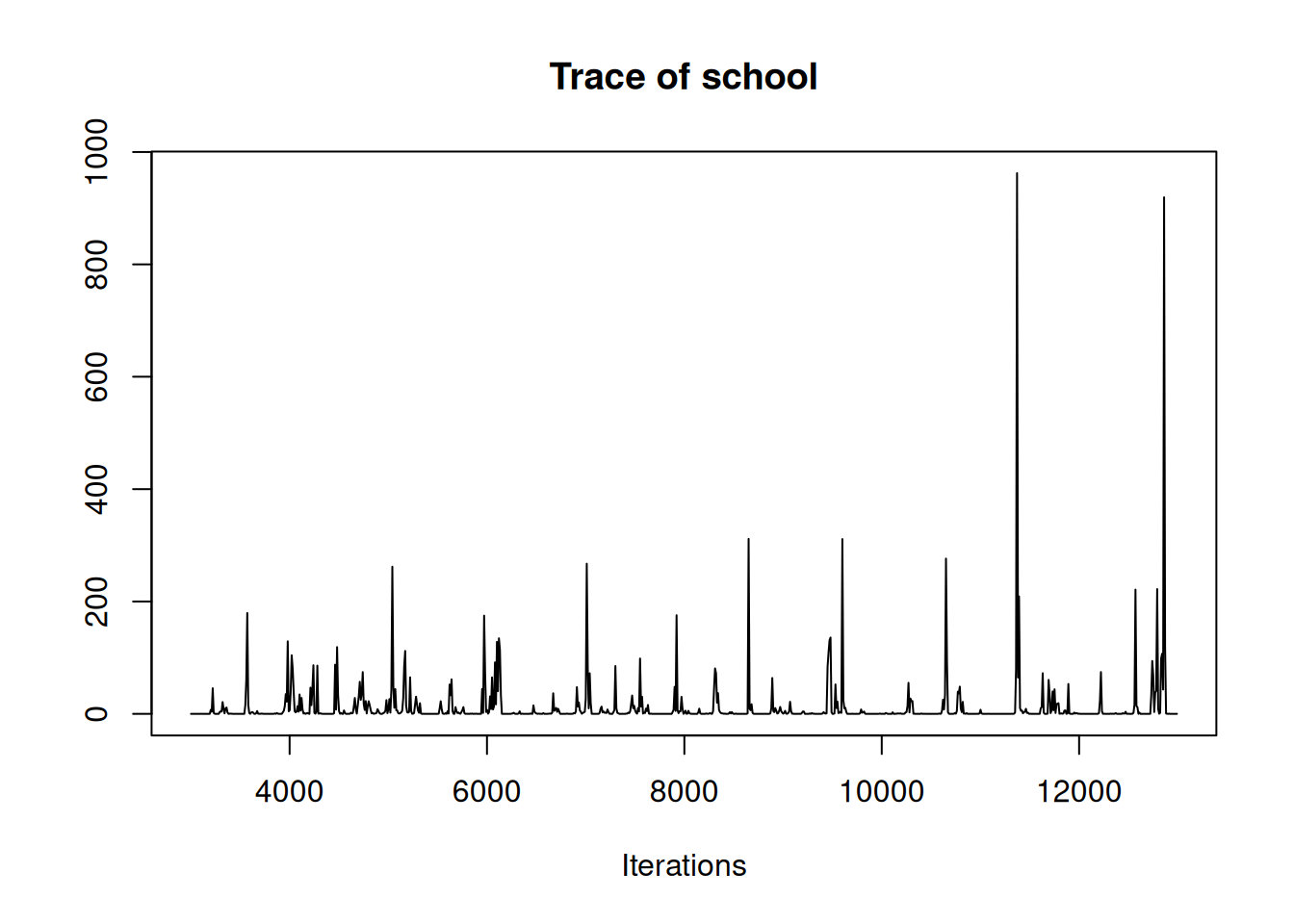
Figure 4.4: MCMC trace for the variance in \(\texttt{school}\) effects from model mschool.1 in which an inverse-Wishart prior was used with \(\texttt{V=1}\) and \(\texttt{nu=0.002}.\)
The autocorrelation in the chain is evident and there appears to be a lot of posterior density at zero. These are separate issues. Autocorrelation in the chain is due to algorithmic inefficiencies in sampling the posterior distribution, whereas a lot of posterior density near zero reflects the combined information coming from the data and coming from the prior (Chapter 2). Certainly, some posterior distributions are harder to sample from than others, and the efficiency of the MCMC algorithm may decrease when the posterior is close to zero. But if the chain can be run long enough that these inefficiencies are not consequential, situations where the posterior has ‘too much’ density near zero indicate potential problems with the prior, not algorithmic problems.
4.6.1 \(F\) and folded-\(t\) priors
For the inverse-Wishart prior we specified the parameters \(\texttt{V}\) and \(\texttt{nu}\). The parameters \(\texttt{alpha.mu}\) and \(\texttt{alpha.V}\) can also be specified in the prior, and if \(\texttt{alpha.V}\) is non-zero then parameter expansion is used. These additional parameters specify a prior for the variance, \(\sigma^2_{\texttt{school}}\), that is a non-central scaled F-distribution with the numerator degrees-of-freedom set to one. We can also think about this prior in terms of the standard deviation, \(\sigma_{\texttt{school}}\), which in some ways is more natural, since it is in the same units as the response. The prior distribution for the standard deviation is a folded scaled non-central \(t\). As the length of their names suggest, these two distributions are quite complicated. Regrettably, this complication is exacerbated in \(\texttt{MCMCglmm}\) by specifying the prior through the distribution of the parameter expansion working parameters (See Section ??). I will leave the full relationship between the prior specification and the \(F\) and \(t\) distributions to the footnote14, and introduce two simplifications here. First, these distributions have three free parameters, yet the prior specification has four. Without loss of generality we will use \(\texttt{V}=1\) throughout. Then, \(\texttt{alpha.V}\) specifies the scale of the \(F\) prior for the variance and \(\sqrt{\texttt{alpha.V}}\) specifies the scale of the \(t\) prior for the standard deviation. Second, since the non-central forms of these distributions are rarely - if ever - used as priors, we will set the non-centrality parameter to zero via \(\texttt{alpha.mu}=0\). For the standard deviation prior this results in the added simplification that the folded-\(t\) becomes the half-\(t\) (essentially a \(t\) with the negative values missing). We are then left with two-parameter distributions with the scale set by \(\texttt{alpha.V}\) and the (denominator) degrees-of-freedom, \(\texttt{nu}\).
Before discussing the properties of the \(F\) and half-\(t\) priors on the posterior distributions of variances and standard deviations, respectively, let’s confirm that parameter expansion does indeed increase efficiency independent of the prior being used. In Section 2.6 we saw that an improper inverse-Wishart distribution with \(\texttt{V}=0\) and \(\texttt{nu}=-1\) is flat for the standard deviation. A half-\(t\) with \(\texttt{nu}=-1\) is also an improper flat prior on the standard deviation irrespective of what is specified for the other parameters. Let’s fit these flat improper priors with and without parameter expansion:
prior.nopx<-list(R=list(V=diag(schools$ve), fix=1),
                      G=list(G1=list(V=1e-16, nu=-1)))

m.nopx<-MCMCglmm(estimate~1, random=~school, rcov=~idh(school):units, data=schools, prior=prior.nopx)
# flat prior on the school standard deviation - no parameter expansion

prior.px<-list(R=list(V=diag(schools$ve), fix=1),
                      G=list(G1=list(V=1e-16, nu=-1, alpha.mu=0, alpha.V=1000^2)))
# note I have set V=1e-16 rather than V=1: with nu=-1, V does not influence the prior

m.px<-MCMCglmm(estimate~1, random=~school, rcov=~idh(school):units, data=schools, prior=prior.px)
# flat prior on the school standard deviation - with parameter expansion
We can see that these two models are sampling from the same posterior (Figure 4.5) but the efficiency of the algorithm is greater when parameter expansion is used, with an effective posterior sample size of 877 rather than 404.
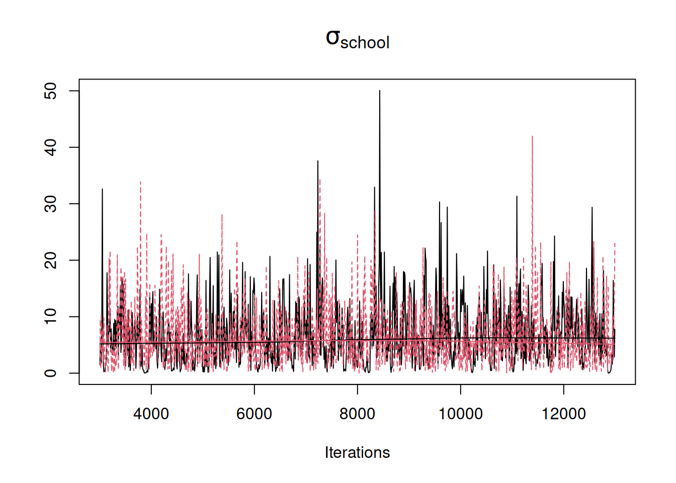
Figure 4.5: MCMC traces for the standard deviation in \(\texttt{school}\) effects. In black is the trace for model m.nopx in which an improper inverse-Wishart prior was used for the variance with \(\texttt{V=0}\) and \(\texttt{nu=-1}\). In red is the trace for model m.px in which an improper \(F_{1,-1}\) prior was used with \(\texttt{nu=-1}\) and $\(\texttt{alpha.V}=1000^2\). Both priors are flat for the standard deviation but m.px employs parameter expansion.
While parameter expansion usually results in more efficient sampling of the posterior, to justify its use, it is important that it also allows us to specify priors with sensible properties. Those with Bayesian scruple may baulk at the use of an improper prior. However, if we specify \(\texttt{nu=1}\) (a half-\(t_1\) or half-Cauchy) we can specify a proper prior that becomes flat for the standard deviation as we increase the scale. Let’s fit a proper half-Cauchy with a scale that is large (relative to the data) - \(\sqrt{\texttt{alpha.V}}=1000\).
prior.mschool.2<-list(R=list(V=diag(schools$ve), fix=1),
                      G=list(G1=list(V=1, nu=1, alpha.mu=0, alpha.V=1000^2)))
# half-Cauchy prior on the standard-deviation with scale 1000

mschool.2<-MCMCglmm(estimate~1, random=~school, rcov=~idh(school):units, data=schools, prior=prior.px)
# flatish prior on the school standard deviation
Overlaying the trace on those obtained under flat improper priors shows that the posterior distributions for \(\sigma_\texttt{school}\) are indistinguishable (Figure 4.6).
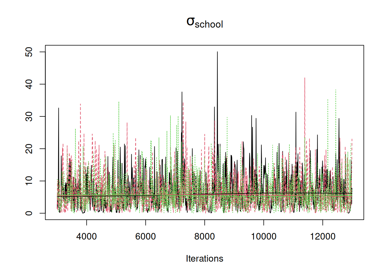
Figure 4.6: MCMC traces for the standard deviation in \(\texttt{school}\) effects. In black is the trace for model m.nopx in which an improper inverse-Wishart prior was used for the variance with \(\texttt{V=0}\) and \(\texttt{nu=-1}\). In red is the trace for model m.px in which an improper \(t_{-1}\) prior was used for the standard deviation with \(\texttt{alpha.V}\) set to \(1000^2\). Both priors are flat for the standard deviation but m.px employs parameter expansion. In green is the trace for model mschool.2 in which a proper half-Cauchy (\(t_{1}\)) with a scale of \(1000\) was used. This prior is almost flat for the standard deviation over the range of values that have reasonable support.
Is a flat(ish) prior on the standard deviation more sensible than the inverse-Wishart prior on the variance we have been using previously (\(\texttt{V}=1\) and \(\texttt{nu}\)=0.002)? The short answer is yes. Setting \(\texttt{nu}\) to be small in the inverse-Wishart is motivated by the idea that having few prior degrees of freedom provides a diffuse prior on the variance. However, as \(\texttt{nu}\) becomes smaller the prior only becomes flat for the log of the variance, and there is a nasty spike at small values for both the variance (Section 2.6) and the standard deviation. However, in some cases, as in the Schools example, the amount of information provided by the data may be so small that a flat prior on the standard deviation might be to vague. In such cases, reducing the scale has been advised, and Gelman (2006) used a scale of 25 for this example:
prior.mschool.3<-list(R=list(V=diag(schools$ve), fix=1),
                      G=list(G1=list(V=1, nu=1, alpha.mu=0, alpha.V=25^2)))

mschool.3<-MCMCglmm(estimate~1, random=~school, rcov=~idh(school):units, data=schools, prior=prior.mschool.3)
When reducing the scale, some care has to be taken that the scale is aligned with the scale of the data. For example, the common ‘default’ recommendation of setting the scale to 5 might prove problematic in this example where the standard deviation of the data exceeds one by some margin:
prior.mschool.4<-list(R=list(V=diag(schools$ve), fix=1),
                      G=list(G1=list(V=1, nu=1, alpha.mu=0, alpha.V=5^2)))

mschool.4<-MCMCglmm(estimate~1, random=~school, rcov=~idh(school):units, data=schools, prior=prior.mschool.4)
The default in brms (Bürkner 2017) is to use a half-\(t\) with 3 degrees of freedom and a scale of 2.5. The tails of this distribution are less ‘heavy’ than the Cauchy and in conjunction with the reduced scale penalise large values more strongly.
prior.mschool.5<-list(R=list(V=diag(schools$ve), fix=1),
                      G=list(G1=list(V=1, nu=3, alpha.mu=0, alpha.V=2.5^2)))

mschool.5<-MCMCglmm(estimate~1, random=~school, rcov=~idh(school):units, data=schools, prior=prior.mschool.5)
When comparing these priors visually we see that they are quite different, despite all having some history as default and/or recommended priors (Figure 4.7).
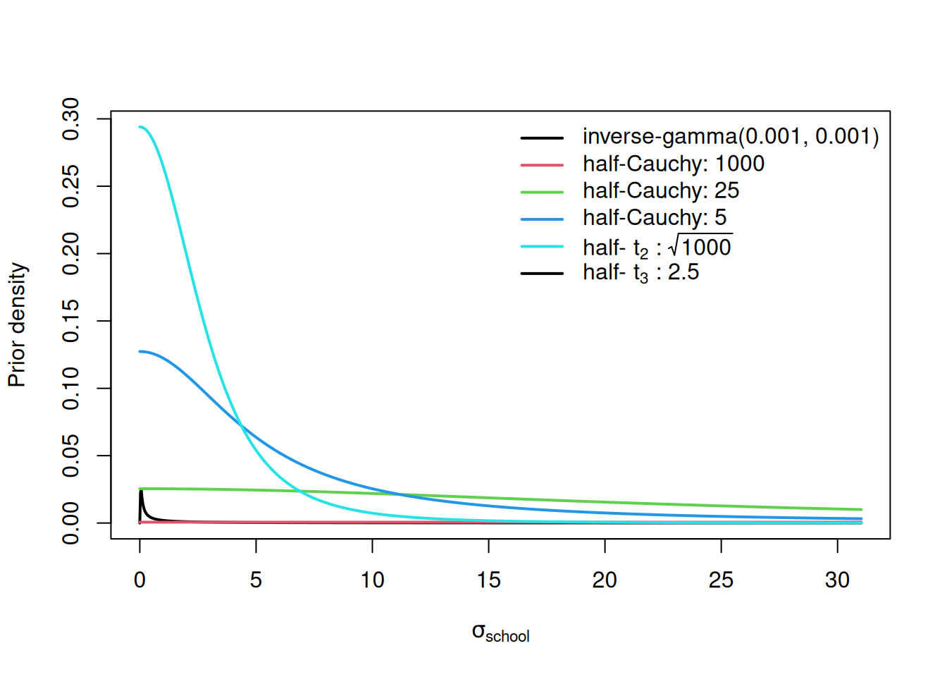
Figure 4.7: Prior probability densities for the standard deviation of \(\texttt{school}\) effects used in the \(\texttt{mschool}\) models \(\texttt{1-5}\). The scale of the half-Cauchy and half-t distributions are given after the colon. Note the inverse-gamma is the prior for the variance - not the standard deviation.
With so little information coming from the data, these priors also have considerable influence on the posterior (Figure 4.8). When \(\texttt{V}\)=1 and \(\texttt{nu}\)=0.002, small values are strongly favoured, and this is also true to a lesser extent for the half-\(t_3\) prior with low scale. As we up the scale and/or reduce the degree-of-freedom to one (the half-Cauchy) the prior becomes flatter and the resulting posteriors are more similar.
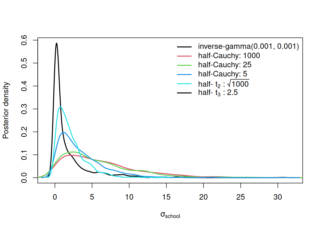
Figure 4.8: Posterior probability densities for the standard deviation of \(\texttt{school}\) effects used in the \(\texttt{mschool}\) models \(\texttt{1-5}\). The priors used in these models are given in the legend with the scale of the half-Cauchy and half-t distributions following the colon. Note the inverse-gamma is the prior for the variance - not the standard deviation.
Figure 4.8 is anxiety-inducing - which prior to use? While I am reluctant to give general advise, in my own work I tend to use a half-Cauchy with a large scale: often \(\sqrt{1000}\) (alpha.V=1000) depending on the scale of the data. However, I try to avoid collecting and analysing data that contains as little information as seen in this example (but see Section 4.9). When this is the case, shifts in the posterior distribution under different priors are often subtle. However, for variances or standard deviations that have support close to zero the spike of the inverse-Wishart/inverse-gamma distribution can cause problems, and for this reason I usually avoid it. The added bonus is faster mixing under parameter expansion. While the prior for the residual variance is restricted to the the inverse-Wishart/inverse-gamma distribution in MCMCglmm (Section 2.6) the data usually contains so much information for the residual variance that prior sensitivity is limited. For models where the random-effect specification defines a (co)variance matrix rather than a scalar variance, see Section 5.3.
4.7 Prior Generators
Even when a user knows which prior they would like to use, it can be rather fiddly generating the prior list, especially when there are many random terms, some of which define (co)variance matrices. In order to simplify the process of prior specification a set of prior generator functions are available in versions >4.0. These functions \(\texttt{IW}\) (inverse-Wishart), \(\texttt{IG}\) (inverse-gamma) and \(\texttt{F}\) (central \(F\) with 1 numerator degree of freedom) take two arguments specifying the parameters of the prior distribution to be used for the variances. The function \(\texttt{tSD}\) can also be used which specifies a half-\(t\)-distribution for the standard deviation. The functions come with default values, but these can be overridden (Table ??). Note that a set parameters can always be chosen such that \(\texttt{IW}=\texttt{IG}\) and \(\texttt{F}=\texttt{tSD}\). The difficult topic of prior specification for (co)variance matrices is covered in Section 5.3 and I’ll leave the documentation of the prior generator functions in this context to then.
| Function | Distribution | Parameter1 | Parameter2 |
|---|---|---|---|
| IW | Inverse-Wishart | V=1 | nu=0.002 |
| IG | Inverse-gamma | shape=0.001 | scale=0.001 |
| F | F with df1=1 | df2=1 | scale=1000 |
| tSD | Half-t (for SD) | df=1 | scale=\(\sqrt{1000}\) |
The prior generator functions can be used to specify the prior for a particular term, or all \(\texttt{G}\) and \(\texttt{R}\) terms. For example, for model mbinom.3 we specified priors for the single residual variance and the two random effect variances:
prior.mbinom.3 = list(R = list(V = 1, fix = 1), G = list(G1 = list(V = 1, nu = 0.002),
    G2 = list(V = 1, nu = 0.002)))
If we wished to use a central \(F_{1,1}\) prior with a scale of a \(1000\) for the variance in the first random term, the long-hand prior would look like:
prior.mbinom.3 = list(R = list(V = 1, fix = 1), G = list(G1 = list(V = 1, nu = 1, alpha.mu=0, alpha.V=1000),
    G2 = list(V = 1, nu = 0.002)))
However, we can also specify this prior as
prior.mbinom.3 = list(R = list(V = 1, fix = 1), G = list(G1 = F(1,1000), G2 = list(V = 1, nu = 0.002)))If we wished to also use the \(F\) prior for the second random term we could either use
or more compactly as:
The prior generators can also be used for the residual variance(s) but because we need to specify additional arguments (\(\texttt{fix}\) in this case) we have to stick with the long-hand version.
4.9 Fixed or Random?
At the start of this Chapter I highlighted the central decision that needs to be made when deciding if an effect should be random or fixed: should a vague prior for the effect (or flat prior in a frequentist analysis) be specified entirely by the analyst (fixed) or should the prior be updated using all data that has relevant information (random)? When put this way, treating something as random would always seem preferable. However, sometimes there is so little relevant information that the benefit of treating an effect as random is outweighed by the cost of the increased complexity. In my experience, when there is a lack of relevant information - the information required to estimate the random-effect variance, \(\sigma^2_u\) - it is almost always because there are only a few levels of the predictor, not because the replication per level is small. This is why people often use the rule-of-thumb that if there are few factor levels (\(<5\)) then we should treat the effects as fixed. In this scenario, even if we had infinite replication at each level, we would still only have fewer than five observations from which to estimate the variance. In such cases a second rule-of-thumb is often satisfied: if the levels are interesting to other people, they are fixed. However, when the two rules-of-thumb are in conflict, people often agonise about the choice. If your data set is of an admirable size, I would argue that it often doesn’t matter what you choose. If you have few levels of a predictor, that probably means you have a lot of replication per level. In these situations, the amount of information coming from observations from that level overwhelm any prior information and so it doesn’t matter whether you say the prior information is vague (fixed) or try and update the prior information from all observations (random).
In my own field, year is often a good example. A field project has ran for less than five years but each year a lot data is collected. Should the year effects be treated as fixed or random? Well there are few levels, suggesting fixed, but the effect of year 2014 (for example) isn’t particularly interesting, suggesting random. People sometimes claim fixed because years haven’t been sampled at random, but this argument shows a deep misunderstanding of what a random effect is. ‘random’ isn’t referring to years being sampled at random, but referring to the fact that we would like to treat year effects as random variables coming from a distribution. If I had observations from many years I would certainly fit year effects as random. However, with few years and a lot of data per year I would treat them as fixed. Let’s consider a data-set I collected and that I use for teaching:
##   tarsus_mm bird_id sex year nest_orig nest_rear day_hatch
## 1      17.2 L298904   F 2011     11_A9     11_A9         0
## 2      17.6 L298903   M 2011     11_A9     11_A9         0
## 3      16.2 L298905   F 2011     11_82     11_A9         0
## 4      17.0 L298901   M 2011     11_82     11_A9         0
## 5      17.3 L298900   M 2011     11_A9     11_A9         1
## 6      16.1 L298902   M 2011     11_82     11_A9         1
\(\texttt{tarsus_mm}\) are the lengths of the tarsus bone in Blue Tit chicks and \(\texttt{year}\) is the year (2011-2014) in which the chicks hatched and I measured them. The remaining variables will not be relevant here. The key point is that \(\texttt{year}\) only has four levels but the number of birds with tarsus measurements is high in each year (between 593 and 854). Let’s fit two models, one where year effects are fixed and one where they are random:
BTtarsus$year<-as.factor(BTtarsus$year)

prior.myear.fixed=list(R=list(V=1, nu=0.002))
myear.fixed<-MCMCglmm(tarsus_mm~year, data=BTtarsus, prior=prior.myear.fixed)

prior.myear.random=list(R=list(V=1, nu=0.002), G=list(G1=list(V=1, nu=1, alpha.mu=0, alpha.V=1000)))
myear.random<-MCMCglmm(tarsus_mm~1, random=~year, data=BTtarsus, pr=TRUE, prior=prior.myear.random)
If we plot the posterior distribution for the estimated year means we can see that they are extremely similar (Figure 4.9).
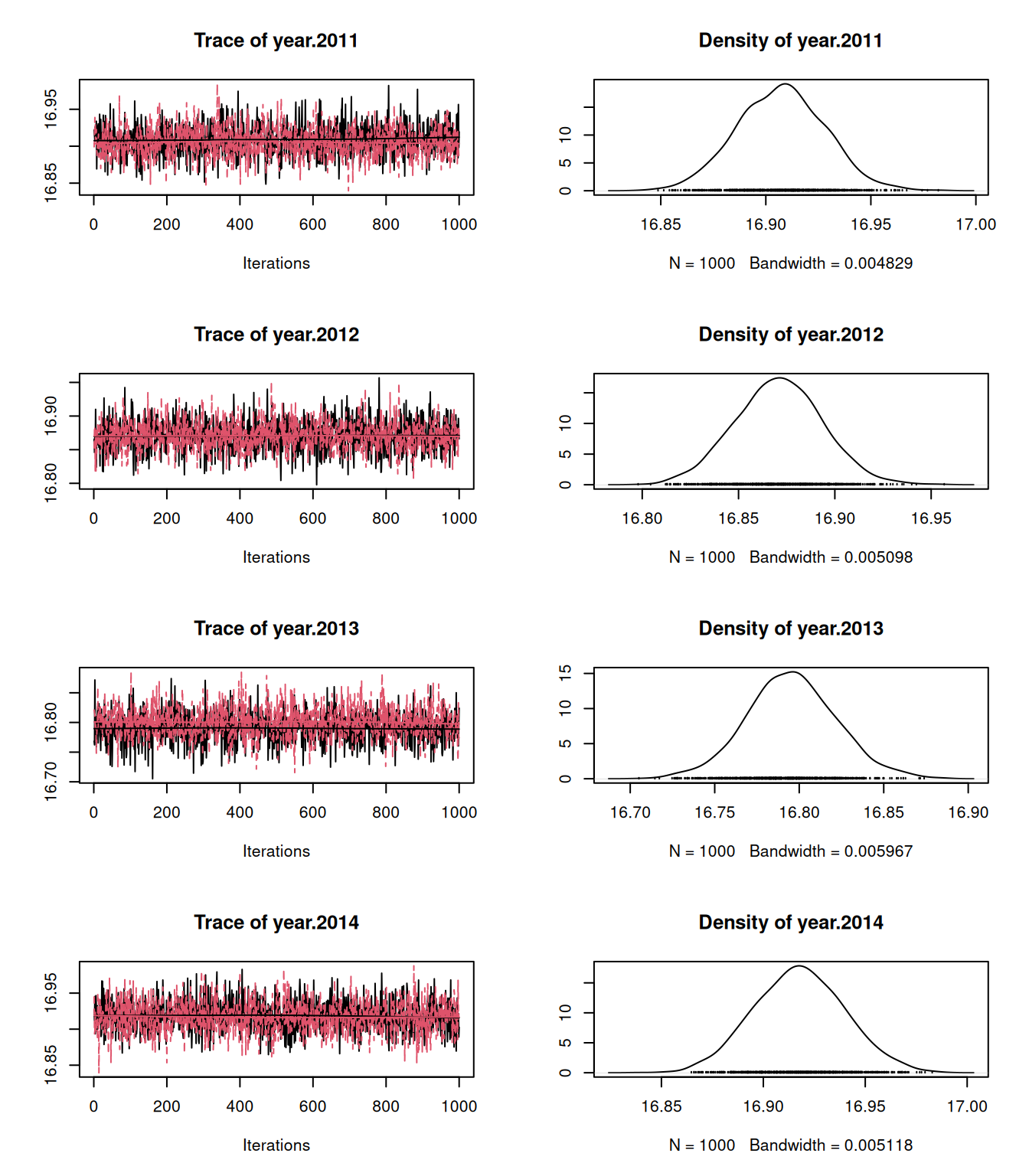
Figure 4.9: MCMC traces for the estimated year means when year effects are treated as fixed (black) or random (red). Because the amount of replication per year is high the posterior distributions are very similar
With a flatish prior on the standard deviation of year effects (half-Cauchy with scale \(\sqrt{1000}\)) the posterior distribution is, for those familiar with Blue Tit tarsus lengths, hopeless uncertain (Figure 4.10). A standard deviation of 0.5 has some support. This implies that some years we expect some seriously stumpy Blue Tits and in other years we expect some seriously leggy Blue Tits. But a standard deviation of 0.05 also has some support and this implies that tarsus length hardly varies from year-to-year. In such cases we might as well admit that we cannot estimate the between year variability with sufficient precision even though we can infer with precision the effect of the handful of years we have measurements for. When this is the case, we may as well treat the effects as fixed.
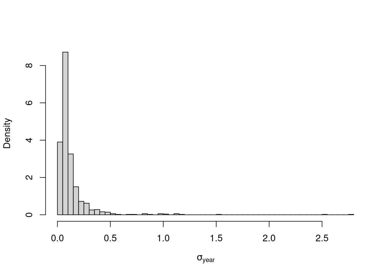
Figure 4.10: Posterior distribution for the standard deviation of year effects from model prior.myear.random.
References
If we assumed the distribution was Laplace (back to back exponentials) we have the LASSO. If we assumed the distribution was a mixture of normal and Laplace we have the elastic net.↩︎
With the now defunct \(\texttt{family="ordinal"}\) the \(\pi^2/3\) in the denominator for the intra-class correlation would have be replaced by a one which is the link variance for the probit (the variance of the unit normal).↩︎
For the \(F\) prior on the variance, the scale is set by \(\texttt{alpha.V}*\texttt{V}\) and the normalised variance \(\sigma^2_{\texttt{school}}/(\texttt{alpha.V}*\texttt{V})\) follows a non-central F distribution with one numerator degree-of-freedom (\(\texttt{df1}\)), \(\texttt{nu}\) denominator degrees-of-freedom (\(\texttt{df2}\)) and a non-centrality parameter (\(\texttt{ncp}\)) equal to \(\texttt{alpha.mu}^2/\texttt{alpha.V}\). The density of \(\sigma^2_{\texttt{school}}\) is therefore the density of \(\sigma^2_{\texttt{school}}/(\texttt{alpha.V}*\texttt{V})\) in this \(F\) distribution divided by the Jacobian, \(\texttt{alpha.V}*\texttt{V}\) (Section 2.7). For the \(t\) prior on the standard deviation, the scale is set by \(\sqrt{\texttt{alpha.V}*\texttt{V}}\) and the normalised standard deviation \(\sigma_{\texttt{school}}/\sqrt{\texttt{alpha.V}*\texttt{V}}\) follows a folded non-central \(t\) distribution with \(\texttt{nu}\) degrees-of-freedom and non-centrality parameter \(\texttt{alpha.mu}/\sqrt{\texttt{alpha.V}}\). The folding is because we are working with the absolute value of the \(t\) variable and so the density for negative values is reflected onto positive values. The density of \(\sigma_{\texttt{school}}\) is therefore the summed density of \(\sigma_{\texttt{school}}/(\texttt{alpha.V}*\texttt{V})\) and \(-\sigma_{\texttt{school}}/(\texttt{alpha.V}*\texttt{V})\) in this \(t\) distribution divided by the Jacobian, \(\sqrt{\texttt{alpha.V}*\texttt{V}}\). This is all very hard to remember! The density of these distributions can be obtained using the function
dpriorwhich evaluates \(\texttt{x}\) according to the MCMCglmm specification passed as a list to the argument \(\texttt{prior}\). The density of the standard deviation (\(\texttt{sd=TRUE}\)) or the variance (the default - \(\texttt{sd=FALSE}\)) can be obtained. For example,dprior(1/2, prior=list(V=1, nu=1, alpha.mu=0, alpha.V=10^2), sd=TRUE), returns the density of \(\sigma_{\texttt{school}}=1/2\) for a half-\(t\) (since \(\texttt{alpha.mu}=0\)) with one degree-of-freedom and scale 10 (i.e a half-Cauchy with scale 10).↩︎