3 Linear and Generalised Linear Models

3.1 Linear Model (LM)

A linear model is one in which unknown parameters are multiplied by (functions of) observed variables and then added together to give a prediction for the response variable. As an example, lets take the results from a Swedish experiment from the sixties:

The experiment involved enforcing speed limits on Swedish roads on some days, but on other days letting everyone drive as fast as they liked. The response variable (y) is the number of accidents recorded. The experiment was conducted in 1961 and 1962 for 92 days in each year. As a first attempt we could specify the linear model:

y ~ limit + year + day

but what does this mean?

3.1.1 Linear Predictors

The model formula defines a set of simultaneous (linear) equations

\[\begin{array}{cl} E[y\texttt{[1]}] &=\beta_{1}+\beta_{2}(\texttt{limit[1]=="yes"})+\beta_{3}(\texttt{year[1]=="1962"})+\beta_{4}\texttt{day[1]}\\ E[y\texttt{[2]}] &= \beta_{1}+\beta_{2}(\texttt{limit[2]=="yes"})+\beta_{3}(\texttt{year[2]=="1962"})+\beta_{4}\texttt{day[2]}\\ \vdots&=\vdots\\ E[y\texttt{[184]}] &= \beta_{1}+\beta_{2}(\texttt{limit[184]=="yes"})+\beta_{3}(\texttt{year[184]=="1962"})+\beta_{4}\texttt{day[184]}\\ \end{array} \label{SE-eq} \tag{3.1}\]

where the \(\beta\)’s are the unknown coefficients to be estimated, and the variables in \(\texttt{this font}\) are observed predictors. Continuous predictors such as day remain unchanged, but categorical predictors are expanded into a series of binary variables of the form ‘do the data come from 1961, yes or no?’, ‘do the data come from 1962, yes or no?’, and so on for as many years for which there are data.

It is cumbersome to write out the equation for each data point in this way, and a more compact way of representing the system of equations is

\[ E[{\bf y}] = {\bf X}{\boldsymbol{\mathbf{\beta}}} \tag{3.2} \]

where \({\bf X}\) is called a design matrix and contains the predictor information for all observations, and \({\boldsymbol{\mathbf{\beta}}} = [\beta_{1}\ \beta_{2}\ \beta_{3}\ \beta_{4}]^{'}\) is the vector of parameters. Here, \(E[{\bf y}]\) is a vector of the 184 expected values.

X <- model.matrix(y ~ limit + year + day, data = Traffic)
X[c(1, 2, 184), ]

##     (Intercept) limityes year1962 day
## 1             1        0        0   1
## 2             1        0        0   2
## 184           1        1        1  92

The binary predictors do the data come from 1961, yes or no? and there was no speed limit, yes or no? do not appear. These are the first factor levels of year and limit respectively, and are absorbed into the global intercept (\(\beta_{1}\)) which is fitted by default in R. Hence the expected number of accidents for the four combinations (on day zero) are \(\beta_{1}\) for 1961 with no speed limit, \(\beta_{1}+\beta_{2}\) for 1961 with a speed limit, \(\beta_{1}+\beta_{3}\) for 1962 with no speed limit and \(\beta_{1}+\beta_{2}+\beta_{3}\) for 1962 with a speed limit.

The simultaneous equations defined by Equation (3.2) cannot be solved directly because we do not know the left-hand side - expected values of \(y\). We only know the observed value, which we assume is distributed around the expected value with some error. In a normal linear model we assume that these errors (residuals) are normally distributed:

\[{\bf y}-{\bf X}{\boldsymbol{\mathbf{\beta}}} = {\bf e} \sim N(0, \sigma^{2}_{e}{\bf I})\]

\({\bf I}\) is a \(184\times 184\) identity matrix. It has ones along the diagonal, and zeros in the off-diagonals. The zero off-diagonals imply that the residuals are uncorrelated, and the ones along the diagonal imply that they have the same variance (\(\sigma^{2}_{e}\)). Thinking about the distribution of residuals is less helpful when we move on to GLM’s and so I prefer to think about the model in the form:

\[{\bf y}\sim N({\bf X}{\boldsymbol{\mathbf{\beta}}}, \sigma^{2}_{e}{\bf I})\]

and say the response is conditionally normal, with the conditioning on the model (\({\bf X}{\boldsymbol{\mathbf{\beta}}}\)). It is important to note that this is different from saying the response is normal. If having a speed limit had a very strong effect the (marginal) distribution of the response may be bimodal and far from normal, and yet by including speed-limit as a predictor, conditional normality may be achieved.

We could use MCMCglmm to fit this model, but to connect better with what comes next, let’s use glm to estimate \({\bf \beta}\) and \(\sigma^{2}_{e}\) assuming that the number of accidents follow a conditional normal distribution (the MCMCglmm syntax is identical):

m2a.1 <- glm(y ~ limit + year + day, data = Traffic)
summary(m2a.1)

## 
## Call:
## glm(formula = y ~ limit + year + day, data = Traffic)
## 
## Coefficients:
##             Estimate Std. Error t value Pr(>|t|)    
## (Intercept) 21.13111    1.45169  14.556  < 2e-16 ***
## limityes    -3.66427    1.35559  -2.703  0.00753 ** 
## year1962    -1.34853    1.31121  -1.028  0.30511    
## day          0.05304    0.02355   2.252  0.02552 *  
## ---
## Signif. codes:  0 '***' 0.001 '**' 0.01 '*' 0.05 '.' 0.1 ' ' 1
## 
## (Dispersion parameter for gaussian family taken to be 71.80587)
## 
##     Null deviance: 14128  on 183  degrees of freedom
## Residual deviance: 12925  on 180  degrees of freedom
## AIC: 1314.5
## 
## Number of Fisher Scoring iterations: 2

On day zero in 1961 in the absence of a speed limit we expect 21.1 accidents (the intercept). With a speed limit we expect 3.7 fewer accidents and we can quite confidently reject the null-hypothesis of no effect - particularly if we were willing to use a one-tailed test, which seems reasonable. There are 1.3 fewer accidents in 1962, although this could just be due to chance, and for every unit increase in \(\texttt{day}\) the number of accidents is predicted to go up by 0.05. The \(\texttt{day}\) variable is encoded as integers from 1 to 92 with the same \(\texttt{day}\) in different years being comparable (for example, the same day of the week and roughly the same date). If \(\texttt{day}\)’s are evenly spaced throughout the year the \(\texttt{day}\) effect is roughly the effect of increasing calender date by four (365/92) days. The estimate of the residual variance, \(\sigma^2_e\), is the dispersion parameter (71.8).

Because the number of accidents are count data we might worry about the assumption of conditional normality, and indeed the residuals show the typical right skew:

hist(resid(m2a.1))

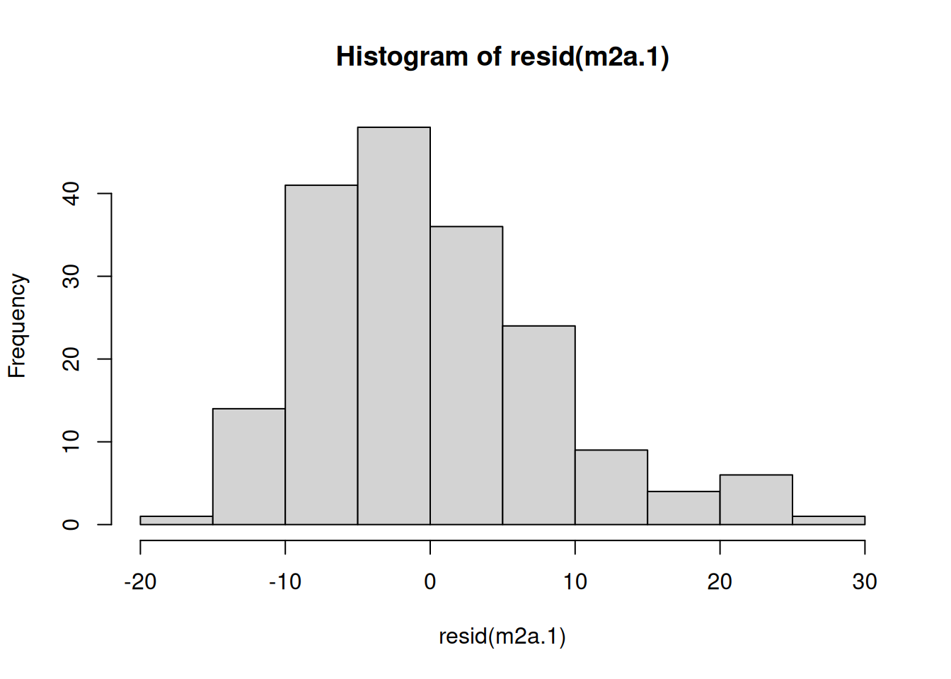
Figure 3.1: Histogram of residuals from model m2a.1 which assumed they followed a Normal distribution.

It’s not extreme, and the conclusions probably won’t change, but we could assume that the data follow some other distribution.

3.2 Generalised Linear Model (GLM)

Generalised linear models extend the linear model to non-normal data. They are essentially the same as the linear model described above, except they differ in two aspects. First, it is not necessarily the mean response that is predicted, but some function of the mean response. This function is called the link function. For example, with a log link we are trying to predict the logged expectation:

\[\textrm{log}(E[{\bf y}]) = {\bf X}{\boldsymbol{\mathbf{\beta}}}\]

or alternatively

\[E[{\bf y}] = \textrm{exp}({\bf X}{\boldsymbol{\mathbf{\beta}}})\]

where \(\textrm{exp}\) is the inverse of the log link function- exponentiating. The second difference is that many distributions are single parameter distributions for which a variance does not need to be estimated because it can be inferred from the mean. For example, we could assume that the number of accidents are Poisson distributed, in which case we also make the assumption that the variance is equal to the expected value. Technically, GLM’s only apply to a restricted set of distributions (those in the exponential family) but \(\texttt{MCMCglmm}\) can accommodate a range of GLM-like models for other distributions (see Table 11.1).

3.3 Poisson GLM

For now we will concentrate on a Poisson GLM with log link (the default link function for the Poisson distribution):

m2a.2 <- glm(y ~ limit + year + day, family = poisson, data = Traffic)
summary(m2a.2)

## 
## Call:
## glm(formula = y ~ limit + year + day, family = poisson, data = Traffic)
## 
## Coefficients:
##               Estimate Std. Error z value Pr(>|z|)    
## (Intercept)  3.0467406  0.0372985  81.685  < 2e-16 ***
## limityes    -0.1749337  0.0355784  -4.917 8.79e-07 ***
## year1962    -0.0605503  0.0334364  -1.811   0.0702 .  
## day          0.0024164  0.0005964   4.052 5.09e-05 ***
## ---
## Signif. codes:  0 '***' 0.001 '**' 0.01 '*' 0.05 '.' 0.1 ' ' 1
## 
## (Dispersion parameter for poisson family taken to be 1)
## 
##     Null deviance: 625.25  on 183  degrees of freedom
## Residual deviance: 569.25  on 180  degrees of freedom
## AIC: 1467.2
## 
## Number of Fisher Scoring iterations: 4

While the sign of the effects are comparable to that seen in the linear model, their numerical values are completely different and the significance of all effects has increased dramatically. Should we worry? The model is defined on the log scale and so to get back to the data scale we need to exponentiate. Exponentiating the intercept gives us the predicted number of accidents on day zero in 1961 without a speed limit:

exp(m2a.2$coef["(Intercept)"])

## (Intercept) 
##    21.04663

which is very close to the intercept in the linear model (21.131), which is reassuring.

To get the prediction for the same day with a speed limit we need to add the \(\texttt{limityes}\) coefficient

exp(m2a.2$coef["(Intercept)"] + m2a.2$coef["limityes"])

## (Intercept) 
##    17.66892

With a speed limit there are expected to be 0.840 as many accidents than if there was no speed limit. This value can be more directly obtained:

exp(m2a.2$coef["limityes"])

##  limityes 
## 0.8395127

and holds true for any given day in either year. The proportional change is identical because the model is linear on the log scale and \(exp(\beta+\dots)=exp(\beta)exp(\dots)\). There is not always a direct relationship with the corresponding coefficients from the linear model but we can reassure ourselves that the parameters have the same qualitative meaning. For example, for \(\texttt{day}\) 0 in 1961 the linear model predicts a drop from 21.1 to 17.5 accidents when a speed limit is in place - around 0.83 as many accidents, comparable to that predicted in the log-linear model.

So in terms of the reported coefficients, the linear model and the Poisson log-linear model are roughly consistent with each other. However, in terms of accurately quantifying the uncertainty in those coefficients the Poisson model has a serious problem - it is very over confident.

3.4 Overdispersion

Most count data do not conform to a Poisson distribution because the variance in the response exceeds the expectation. In the summary to m2a.2 the ratio of the residual deviance to the residual degrees of freedom is 3.162 which means, roughly speaking, there is 3.2 times more variation in our response (after conditioning on the model) than what we expect. This is known as overdispersion and it is easy to see how it arises, and why it is so common.

If the predictor data had not been available to us then the only model we could have fitted was one with just an intercept:

m2a.3 <- glm(y ~ 1, data = Traffic, family = "poisson")
summary(m2a.3)

## 
## Call:
## glm(formula = y ~ 1, family = "poisson", data = Traffic)
## 
## Coefficients:
##             Estimate Std. Error z value Pr(>|z|)    
## (Intercept)  3.07033    0.01588   193.3   <2e-16 ***
## ---
## Signif. codes:  0 '***' 0.001 '**' 0.01 '*' 0.05 '.' 0.1 ' ' 1
## 
## (Dispersion parameter for poisson family taken to be 1)
## 
##     Null deviance: 625.25  on 183  degrees of freedom
## Residual deviance: 625.25  on 183  degrees of freedom
## AIC: 1517.2
## 
## Number of Fisher Scoring iterations: 4

for which the residual variance exceeds that expected by a factor of 3.5. Of course, the variability in the residuals must go up if there are factors that influence the number of accidents, but which we hadn’t measured. It’s likely that in most studies there are things that influence the response that haven’t been measured, and even if each thing has a small effect individually, in aggregate they can cause substantial overdispersion.

3.4.1 Multiplicative Overdispersion

There are two ways of dealing with overdispersion. With glm the distribution name can be prefixed with quasi and a dispersion parameter estimated:

m2a.4 <- glm(y ~ limit + year + day, family = quasipoisson, data = Traffic)
summary(m2a.4)

## 
## Call:
## glm(formula = y ~ limit + year + day, family = quasipoisson, 
##     data = Traffic)
## 
## Coefficients:
##              Estimate Std. Error t value Pr(>|t|)    
## (Intercept)  3.046741   0.067843  44.909  < 2e-16 ***
## limityes    -0.174934   0.064714  -2.703  0.00753 ** 
## year1962    -0.060550   0.060818  -0.996  0.32078    
## day          0.002416   0.001085   2.227  0.02716 *  
## ---
## Signif. codes:  0 '***' 0.001 '**' 0.01 '*' 0.05 '.' 0.1 ' ' 1
## 
## (Dispersion parameter for quasipoisson family taken to be 3.308492)
## 
##     Null deviance: 625.25  on 183  degrees of freedom
## Residual deviance: 569.25  on 180  degrees of freedom
## AIC: NA
## 
## Number of Fisher Scoring iterations: 4

glm uses a multiplicative model of overdispersion and so the estimate of the dispersion parameter is roughly equivalent to how many times greater the variance is than expected, after taking into account the predictor variables. You will notice that although the parameter estimates have changed very little, the standard errors have gone up and the significance gone down. Overdispersion, if not dealt with, can result in extreme anti-conservatism. For example, the second lowest number of accidents (8) occurred on \(\texttt{day}\) 91 of 1961 without a speed limit. Our model predicts this should have been the second worst day for accidents over the whole two years, and the probability of observing 8 or less accidents on this day is predicted to be approximately 3 in a 100,000:

ppois(8, exp(m2a.2$coef["(Intercept)"] + 91 * m2a.2$coef["day"]))

## [1] 3.195037e-05

If we did not accommodate the overdispersion, anything additional we put in in the model that could potentially explain such an improbable occurrence would come out as significant even if in reality it wasn’t important. This is because there simply isn’t any flexibility in the null model to accommodate such occurrences. For example, if the extreme value happened to be associated with a particular level of a categorical predictor or happened to be associated with an extreme value of some continuous predictor, then the coefficients associated with these predictors may well come out as significant. However, under a more plausible null model the extreme observations may not be too surprising and there may be little support for the predictors having an effect on the response. A more plausible model, and one that we’ve alluded to, would be to allow the number of accidents to vary across sampling points due to unmeasured variables. This would allow the variation in the number of accidents to exceed the predicted mean based on the measured variables (the assumption of the standard Poisson).

3.4.2 Additive Overdispersion

I believe that a model assuming all relevant variables have been measured or controlled for, should not be the default model, and so when you specify family=poisson in \(\texttt{MCMCglmm}\), overdispersion is always dealt with⁴. However, \(\texttt{MCMCglmm}\) does not use a multiplicative model, but an additive model.

prior <- list(R = list(V = 1, nu = 0.002))
m2a.5 <- MCMCglmm(y ~ limit + year + day, family = "poisson", data = Traffic, prior = prior,
    pl = TRUE)

The element Sol contains the posterior distribution of the coefficients of the linear model, and we can plot their marginal distributions:

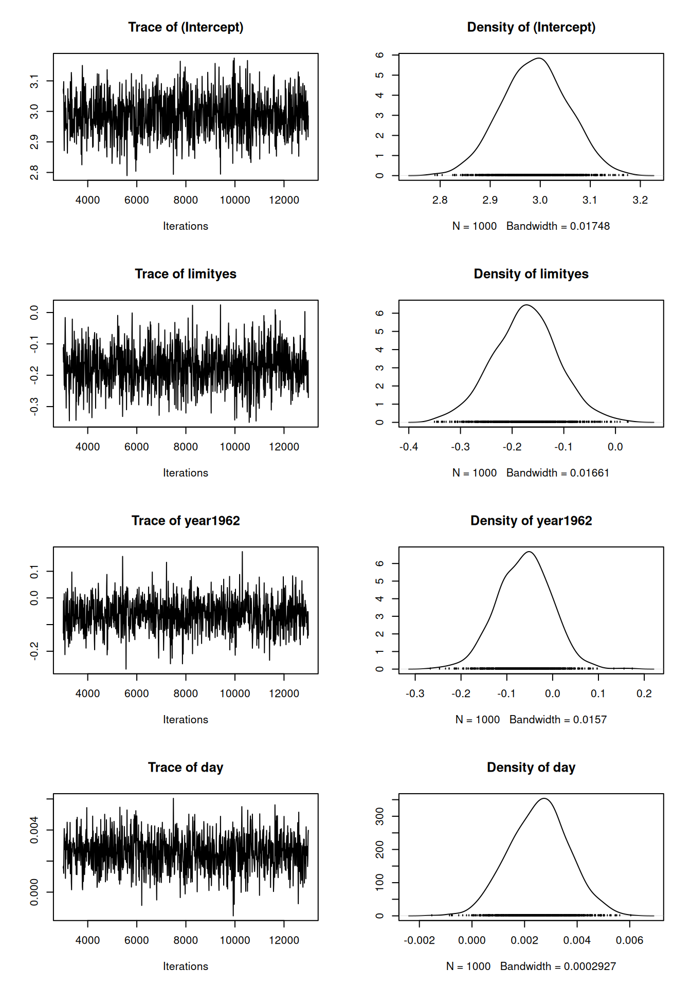
Figure 3.2: MCMC summary plot for the coefficients from a Poisson glm (model m2a.5).

Note that the posterior distribution for the year1962 spans zero, in agreement with the quasipoisson glm model, and that in general the estimates for the two models (and their uncertainty - see Section 2.4.2) are broadly similar:

summary(m2a.4)

## 
## Call:
## glm(formula = y ~ limit + year + day, family = quasipoisson, 
##     data = Traffic)
## 
## Coefficients:
##              Estimate Std. Error t value Pr(>|t|)    
## (Intercept)  3.046741   0.067843  44.909  < 2e-16 ***
## limityes    -0.174934   0.064714  -2.703  0.00753 ** 
## year1962    -0.060550   0.060818  -0.996  0.32078    
## day          0.002416   0.001085   2.227  0.02716 *  
## ---
## Signif. codes:  0 '***' 0.001 '**' 0.01 '*' 0.05 '.' 0.1 ' ' 1
## 
## (Dispersion parameter for quasipoisson family taken to be 3.308492)
## 
##     Null deviance: 625.25  on 183  degrees of freedom
## Residual deviance: 569.25  on 180  degrees of freedom
## AIC: NA
## 
## Number of Fisher Scoring iterations: 4

With additive overdispersion the linear predictor includes a ‘residual’, for which a residual variance is estimated (hence our prior specification).

\[E[{\bf y}] = \textrm{exp}({\bf X}{\boldsymbol{\mathbf{\beta}}}+{\bf e})\]

At this point it will be handy to represent the linear model in a new way:

\[{\bf l} = {\boldsymbol{\mathbf{\eta}}}+{\bf e}\]

where \({\bf l}\) is a vector of latent variables (\(\textrm{log}(E[{\bf y}])\) in this case) and \({\boldsymbol{\mathbf{\eta}}}\) is the usual symbol for the linear predictor (\({\bf X}{\boldsymbol{\mathbf{\beta}}}\)). The data we observe are assumed to be Poisson variables with expectation equal to the exponentiated latent variables:

\[{\bf y} \sim Pois(\textrm{exp}({\bf l}))\]

Note that the latent variable does not exactly predict \(y\), as it would if the data were Normal, because there is additional variability in the Poisson process⁵. In the call to \(\texttt{MCMCglmm}\) I specified pl=TRUE to indicate that I wanted to store the posterior distributions of the latent variables (also known as the liabilities). This is not usually necessary and can require a lot of memory (we have 1000 posterior samples for each of the 182 data points). However, as an example we can obtain the posterior mean residual for data point 92 which is the data from \(\texttt{day}\) 92 in 1961 when there was no speed limit:

lat92 <- m2a.5$Liab[, 92]
# posterior distribution of the 92nd latent variable (liability)

eta92 <- m2a.5$Sol[, "(Intercept)"] + m2a.5$Sol[, "day"] * Traffic$day[92]
# posterior distribution of X\beta for the 92nd observation

resid92 <- lat92 - eta92
# posterior distribution of e for the 92nd observation

mean(resid92)

## [1] -0.1341791

# posterior mean of e for the 92nd observation

This particular observation has a negative expected residual indicating that the probability of getting injured was less than expected for this particular realisation of that \(\texttt{day}\) in that year without a speed limit. If that combination of predictors (\(\texttt{day}\)=92, \(\texttt{year}\)=1961 and \(\texttt{limit}\)=\(\texttt{no}\)) could be repeated it does not necessarily mean that the actual number of accidents would always be less than expected, because it would follow a Poisson distribution with a mean equal to exp(lat92) (21.974).

Like residuals in a standard linear model, the residuals are assumed to be independently and normally distributed with an expectation of zero and an estimated variance. If the residual variance was zero then \({\bf e}\) would be a vector of zeros and the model would conform to the standard Poisson GLM. However, the posterior distribution of the residual variance is located well away form zero:

plot(m2a.5$VCV)

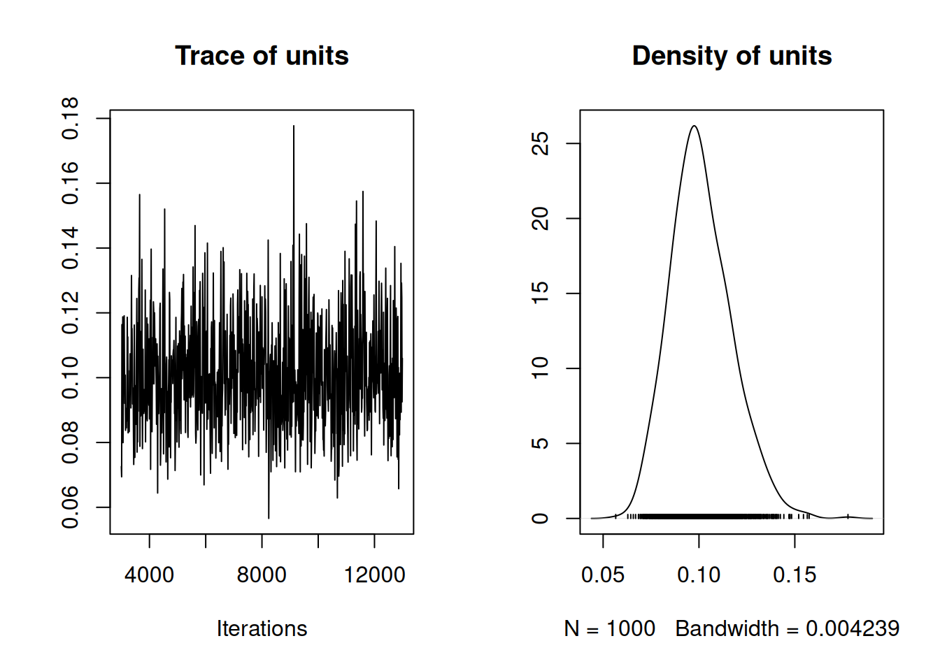
Figure 3.3: MCMC summary plot for the residual (units) variance from a Poisson glm (model m2a.5). The residual variance models any overdispersion, and a residual variance of zero would imply that the response conforms to a standard Poisson.

3.5 Prediction in GLM

To get the expected number of accidents for the 92nd observation we simply exponentiated the latent variable: exp(lat92). However, it is important to realise that this is the expected number had the residual been exactly equal to the observed residual for that observation (resid92): we are calculating the expected number conditional on the set of unmeasured variables that affected that particular realisation of \(\texttt{day}\) 92 in 1961 without a speed limit. When calculating a prediction we usually aim to average over these residuals (or random effects - see 4.2) since we would like to know what the average response would be for observations made on a \(\texttt{day}\) of type 92 in 1961 without a speed limit. On the log-scale the expectation is simply the linear predictor (\(\eta\)):

\[ log(E_e[y]) = E_e[l] = E_e[\eta+e] = \eta+E_e[e]=\eta \]

since the residuals have zero expectation (here I have subscripted the expectation with the variable we are averaging over). The predict function can be applied to MCMCglmm objects and if we specify type="terms" we get the prediction of the link scale - the log scale in this case:

predict(m2a.5, type = "terms")[92]

## [1] 3.224037

which is equal to the posterior mean of eta92 obtained earlier. We can see this visually in Figure 3.4 where I have plotted the distribution of the latent variable on a \(\texttt{day}\) of type 92 in 1961 without a speed limit.

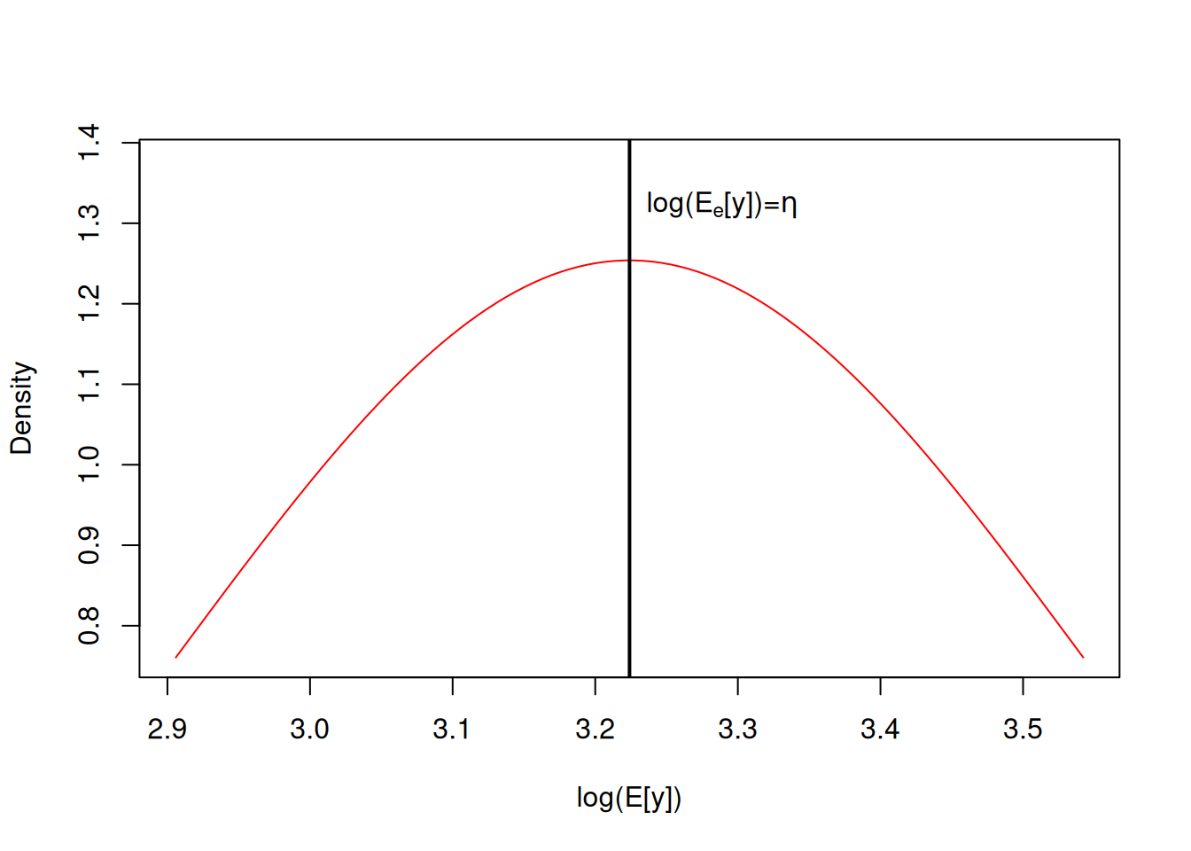
Figure 3.4: The predicted distribution for the average number of accidents on the log scale for a \(\texttt{day}\) of type 92 in 1961 without a speed limit (in red). On the log scale the distribution is assumed to be normal around the linear predictor (\(\eta=\)) with a variance of \(\sigma^{2}_e\). As a consequence the mean, median and mode of the distribution are equal to the linear predictor on the log scale.

To get the prediction on the data scale (i.e. in terms of the actual expected number of accidents) it is tempting to think we could just calculate exp(eta92). However, this is the expected number of accidents had the residual been exactly zero. If we wish to average over the residuals we require:

\[ E_e[y] = E_e[\textrm{exp}(l)] = E_e[\textrm{exp}(\eta+e)] \]

and because exponentiation is a non-linear function this average will deviate from \(\textrm{exp}(\eta)\) (Figure 3.5.

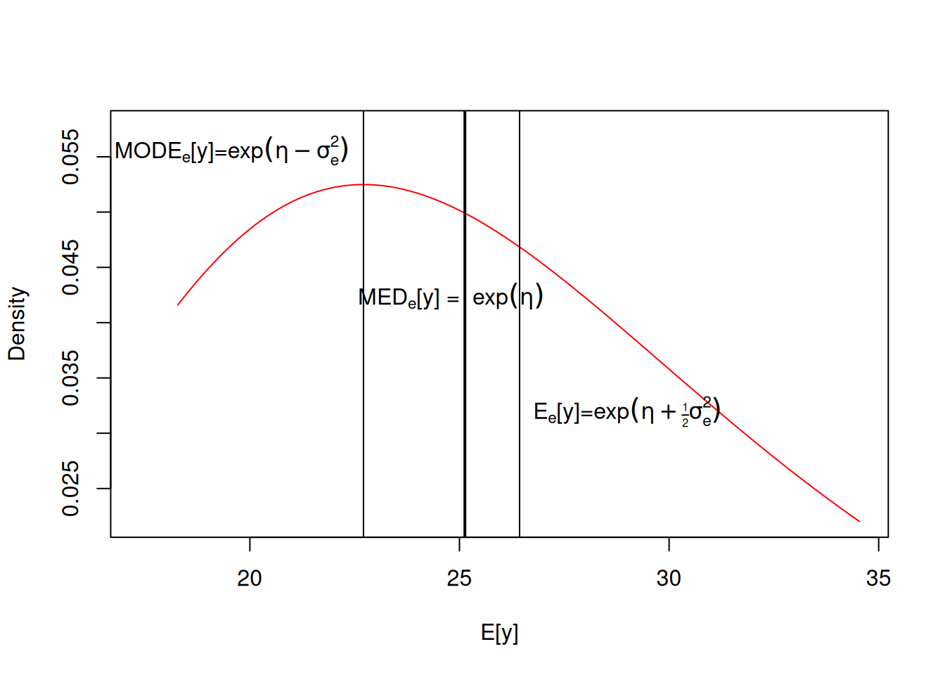
Figure 3.5: The predicted distribution for the average number of accidents on the data scale for a \(\texttt{day}\) of type 92 in 1961 without a speed limit (in red). On the log scale the distribution is assumed to be normal around the linear predictor (\(\eta\)) with a variance of \(\sigma^{2}_e\) (see 3.4). However when transforming to the data scale (by exponentiating) the symmetry is lost and the different measures of central tendency do not coincide. Since the residuals are normal on the log scale, the distribution on the data scale is log-normal and so analytical solutions exist for the mean, mode and median.

To obtain predictions on the data scale we can specify type="response" (the default) when using predict:

predict(m2a.5)[92]

## [1] 26.48956

which is slightly greater than exp(eta92) (25.183). For all link-functions, the median value on the data scale can be easily calculated by taking the inverse-link transform of the linear predictor. However, obtaining the mean and mode is often more challenging than it is for log-link, and numerical integration or approximations are required.

The predict function is returning a single number for observation 92 yet the model object contains 1,000 samples from the posterior distribution of all model parameters. This is because the predict function returns the posterior mean of the predicted value. Since we have the complete posterior distribution we can also place a 95% credible interval on the prediction (see Section 2.4.2):

predict(m2a.5, interval = "confidence")[92, ]

##      fit      lwr      upr 
## 26.48956 23.27675 30.10716

3.5.1 Posterior Predictive Distribution

In some cases we would like to visualise or summarise aspects of the predictive distribution other than the mean. The complete predictive distribution is hard to work with, but the simulate function allows you to draw samples from the predictive distribution. The default is to generate a sample using a random draw from the posterior distribution, resulting in a draw from what is known as the posterior predictive distribution:

ypred <- simulate(m2a.5)

We can use these simulated values to characterise any aspect of the predictive distribution we want. For example, we can obtain quantiles and compare them to the quantiles of the actual data to see how well the model captures aspects of the observed marginal distribution:

qqplot(ypred, Traffic$y)
abline(0, 1)

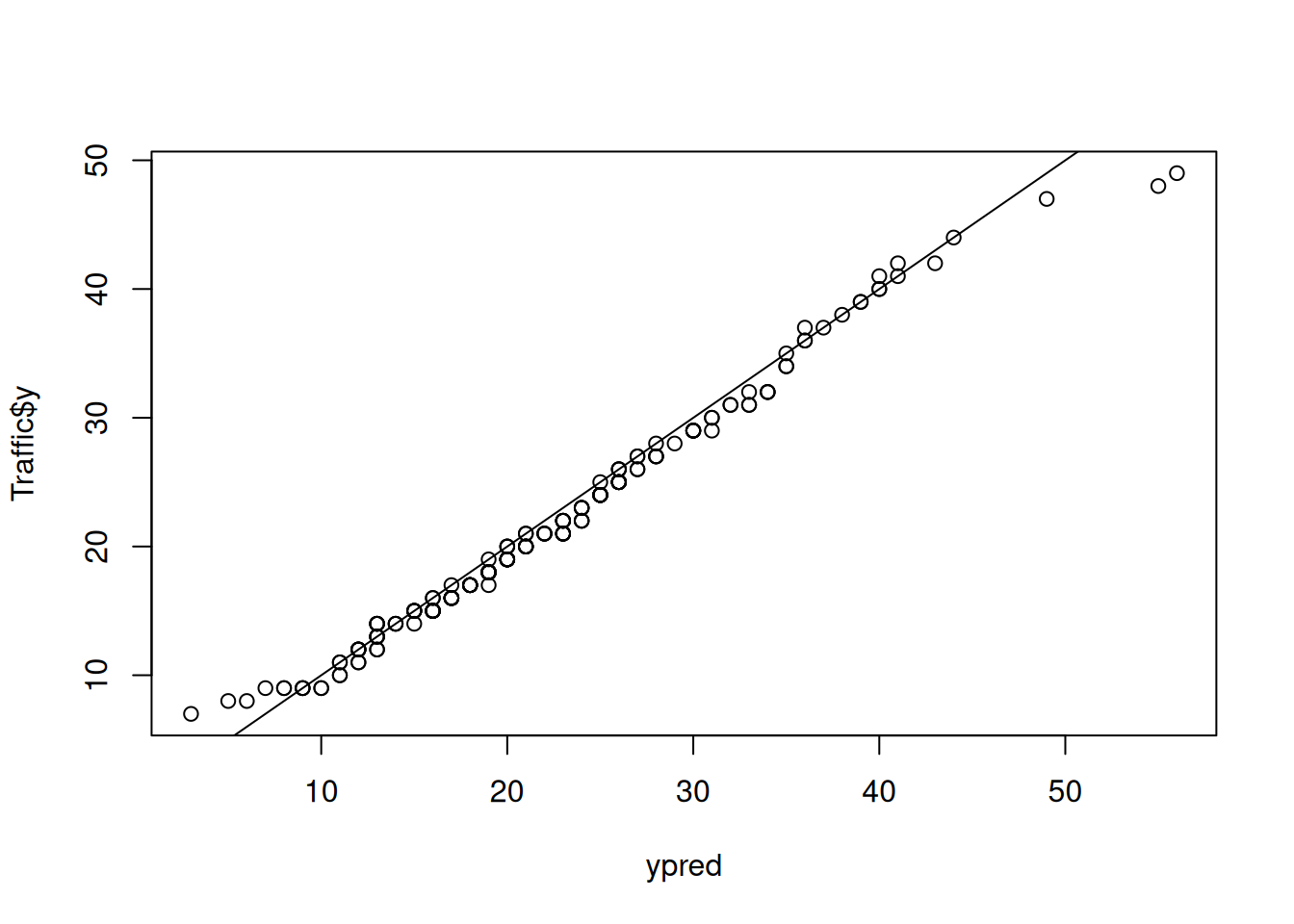
Figure 3.6: qq-plot of the posterior predictive distribution and the data distribution

Not too bad, although the predictive distribution perhaps has greater support for extreme values than are observed. If we merely wish to know the interval in which some specified percentage of the data are predicted to lie, we can also use the predict function but with interval="prediction". By default the 95% (highest posterior density) interval is calculated using as many simulated samples as there are saved posterior samples. For the 92nd observation the prediction interval is

predict(m2a.5, interval = "prediction")[92, ]

##    fit    lwr    upr 
## 26.696 10.000 47.000

Note that the reported mean (fit) differs from that returned by interval="confidence" due to Monte Carol error only.

3.6 Binomial and Bernoulli GLM

The general concepts introduced for the Poisson GLM extend naturally to Binomial data, albeit with a different link function. However, it is worth spending a little time exploring a Binomial GLM as I think overdispersion, and how we deal with it, is easier to understand with binomial data. However, we’ll also see how the ‘residuals’ defined earlier for capturing overdispersion complicate the analysis of Bernoulli data and result in MCMcglmm using a non-standard parameterisation.

The Binomial distribution has two parameters - the number of trials \(n\) and the probability of success, \(p\). In a Binomial GLM the number of trials is assumed known leaving only \(p\) to be estimated from the number of trials that are ‘successes’ or ‘failures’. When family="binomial" is specified (or equivalently family="multinomial2"⁶) MCMCglmm uses the standard link function for the Binomial - the logit link - and the logit probability of success is modelled as

\[log\left(\frac{p}{1-p}\right) = l = \eta+e\]

The logit transform takes a probability and turns it into a log odds ratio. If we want to get back to the probability we use the inverse of the logit transform:

\[p = \frac{exp(l)}{1+exp(l)}\]

The logit link is actually the quantile function for the logistic distribution and so is available as the function qlogis. The inverse of a quantile function is a cumulative distribution function and so the inverse-logit transform is plogis.

To introduce the Binomial GLM we will analyse some data I collected on how grumpy my colleagues look. I took two photos (\(\texttt{photo}\)) of 22 people (\(\texttt{person}\)) working in the Institute of Evolution and Ecology, Edinburgh. In one photo the person was happy and in the other they were grumpy (\(\texttt{type}\)). 122 respondents gave a score between 1 and 10 indicating how grumpy they thought each person looked in each photo (with 10 being the most grumpy).

data(Grumpy)
Grumpy[c(1:3, 44), ]

##           y  l5  g5   type photo   person age ypub
## 1  4.032787 101  21 grumpy  4511   ally_p  38   13
## 2  3.081967 113   9  happy  4512   ally_p  38   13
## 3  7.885246  15 107 grumpy  4521 darren_o  38   16
## 44 3.798319 105  14  happy  4516  laura_r  34   10

\(\texttt{y}\) gives the average score given by the 122 respondents. The number of respondents giving a photo a score of five or less (\(\texttt{l5}\)) or more than five (\(\texttt{g5}\)) is also recorded in addition to the person’s age (\(\texttt{age}\)) and a proxy for how long they had been academia - the number of years since they published their first academic paper (\(\texttt{ypub}\)). Here, we will model the probability of getting a grumpy score greater than five as a function of whether the person was happy or grumpy and how long they had been in academia. As with glm, successes should be in the first column of the response, and failures in the second:

mbinom.1 <- MCMCglmm(cbind(g5, l5) ~ type + ypub, data = Grumpy, family = "binomial",
    pl = TRUE)
summary(mbinom.1)

## 
##  Iterations = 3001:12991
##  Thinning interval  = 10
##  Sample size  = 1000 
## 
##  DIC: 5377.999 
## 
##  R-structure:  ~units
## 
##       post.mean l-95% CI u-95% CI eff.samp
## units     1.348   0.7597    1.947     1000
## 
##  Location effects: cbind(g5, l5) ~ type + ypub 
## 
##             post.mean l-95% CI u-95% CI eff.samp  pMCMC    
## (Intercept)  -0.72025 -1.67538  0.05147     1000  0.094 .  
## typehappy    -1.28167 -1.97027 -0.59820     1000 <0.001 ***
## ypub          0.02064 -0.00613  0.05175     1105  0.156    
## ---
## Signif. codes:  0 '***' 0.001 '**' 0.01 '*' 0.05 '.' 0.1 ' ' 1

The model coefficients are most easily interpreted after exponentiating as they then give the proportional change in the odds ratio. The odds of having a score greater than five is exp(-1.282)=0.278 times lower when happy, as expected. The odds increases by a factor exp(0.021)=1.021 for each year in academia. When the coefficient is small in magnitude like this, you can get a rough estimate by looking directly at the coefficient: 0.021 roughly translates into a 2.1% increase and -0.021 would translate into a 2.1% decrease⁷. The \(\texttt{units}\) (residual) variance is also large with credible intervals that are far from zero.

3.6.1 Overdispersion

As with overdispersion in the Poisson model, this excess variation can be attributed to predictors that are not included in the model but cause the probability of success to vary over observations (photos in this case). For example, the 3rd and 25th observation have the same values for every predictor

Grumpy[c(3, 25), ]

##           y l5  g5   type photo   person age ypub
## 3  7.885246 15 107 grumpy  4521 darren_o  38   16
## 25 5.319672 73  49 grumpy  4527  craig_w  38   16

and so in the absence of overdispersion these parameters would result in a predicted probability of success of

\[p = \textrm{plogis}(\beta_{\texttt{(Intercept)}}+\beta_{\texttt{typehappy}}\times0+\beta_{\texttt{ypub}}\times16)=0.404 \label{plogis-eq} \tag{3.3}\]

Given there were 122 respondents (trials) we can calculate the two values between which the number of successes is expected to fall 95 % of the time.

qbinom(c(0.025, 0.975), size = 122, prob = p)

## [1] 39 60

While photo \(\texttt{4527}\) is well within the range with 49 successes, the number of respondents giving photo \(\texttt{4521}\) is substantially higher (107) - it’s an outlier. In Figure 3.7 the two photos are shown and it is clear why their underlying probabilities may deviate from that predicted. Most obviously the two photos are of different people and people vary in how grumpy they look. Since we have two photos per person we could (and should) estimate \(\texttt{person}\) effects, however this is best done by treating these effects as random, which we will cover later, in Section 4.1. Even if \(\texttt{person}\) effects were fitted there’s also likely to be a whole host of observation-level (photo-specific) effects that are not captured in the model such as whether the person had their eyes closed or was wearing a dreary grey fleece.

Figure 3.7: Photo 4521 (left) and photo 4527 (right). For the predictors fitted in model mbinom.1, these photos have the same values (\(\texttt{type}=\texttt{grumpy}\) and \(\texttt{ypub}=16\) years)

If we include the ‘residuals’ when calculating the predicted probability for these two photos we can see that indeed their probabilities are quite different:

mean(plogis(mbinom.1$Liab[, 3]))

## [1] 0.8621967

# predicted probability for photo 4521
mean(plogis(mbinom.1$Liab[, 25]))

## [1] 0.4001446

# predicted probability for photo 4527

3.6.2 Prediction

When calculating the predicted probability in the absence of the residuals in Equation (3.3) I was careful to say that the prediction assumed an absence of overdispersion. However, when overdispersion is present we need to average over the distribution of the residuals in order to get an average. As we saw in the log-linear Poisson model, because the inverse-link function (plogis) is non-linear the average of \(E_e[\texttt{plogis}(\eta+e)]\) is different from \(\texttt{plogis}(E_e[\eta+e])=\texttt{plogis}(\eta)\). Unlike the Poisson log-linear model this expectation cannot be calculated analytically and the predict function by default numerically evaluates the integral:

\[\int_l \texttt{plogis}(l)f_N(l | \eta, \sigma^2_e)dl\]

where \(f_N\) is the probability density function of the normal. For each of the 44 observations this is done 1,000 times (the number of saved posterior samples) to get the posterior mean prediction and can be very slow (it is actually faster to fit the model). The number reported by predict is \(np\) rather than \(p\) and so to get the predicted probability for a photo of someone who has grumpy and had been publishing for 16 years we can get the prediction for the 3rd observation and divide by the number of trials (122):

predict(mbinom.1)[3]/122

## [1] 0.4243498

A little different from \(\texttt{plogis}(\eta)=\) 0.404. For the binomial with logit link, analytical approximations have been developed in Diggle et al. (2004) and McCulloch and Searle (2001) which are considerably faster and reasonably accurate:

predict(mbinom.1, approx = "diggle")[3]/122

## [1] 0.4210936

predict(mbinom.1, approx = "mcculloch")[3]/122

## [1] 0.4255396

3.6.3 Bernoulli GLM

Bernoulli data are a special case of the Binomial in which the number of trials is equal to one and so either a success or a failure is observed. To explore a Brenoulli model we can take our average Grumpy scores and simply dichotomise them into whether the average score was five or less or more than five:

Grumpy$mean5 <- Grumpy$y > 5

If we fit a binomial model to these data in MCMCglmm it has exactly the same form as before (although a single column of outcomes can be passed). But importantly, for Bernoulli data there is no information to estimate the residual variance. This does not necessarily mean that variation in the probability of success across observations is absent, only that we can’t estimate it. For example, imagine we took 100 people who had been publishing for 16 years and took a photograph of them when they were grumpy. Let’s say the probability that the mean score for such photos exceeded 5 was 0.5. If the probability for all photos was exactly 0.5 (i.e. the probability of success did not vary over observations) then we expect 50 success and 50 failures across our observations. However, imagine the case where the probability of success was 100% for 50 photos and 0% for 50 photos (i.e. the probability of success varies considerably over observations). We would also expect 50 success and 50 failures, and so the distribution of successes with and without variation in the underlying probability would be identical. In the absence of information most software sets the ‘residual’ variance to zero (i.e. the probability of success dose not vary over observations), but it is important to understand that this is a convenient but arbitrary choice. Given this, it is desirable that any conclusions drawn from the model do not depend on this arbitrary choice. Worryingly, both the location effects (fixed and random) and variance components are completely dependent on the magnitude of the residual variance. MCMCglmm allows the user to fix the residual variance at a value of their choice, but unfortunately a value of zero results in a chain that will not mix and so I usually fix the residual variance to one⁸:

prior.mbern.1 = list(R = list(V = 1, fix = 1))
mbern.1 <- MCMCglmm(mean5 ~ type + ypub, family = "binomial", data = Grumpy, prior = prior.mbern.1)

However, it would have been equally valid to fixed the residual variance at three:

prior.mbern.2 = list(R = list(V = 3, fix = 1))
mbern.2 <- MCMCglmm(mean5 ~ type + ypub, family = "binomial", data = Grumpy, prior = prior.mbern.2)

and if we compare the MCMC traces for the coefficients we can see that we are sampling different posterior distributions (Figure 3.8).

plot(mcmc.list(mbern.1$Sol, mbern.2$Sol), density = FALSE)

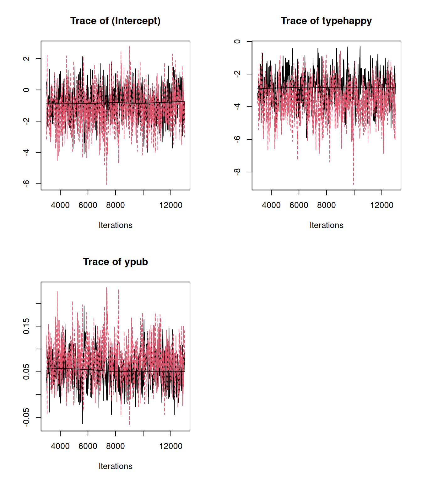
Figure 3.8: MCMC trace for coefficients of a Bernoulli GLM from two models (mbern.1 in black and mbern.2 in red). The data and model structure are identical but in mbern.1 the residual variance was set to one and in mbern.2 the residual variance was set to three. The data provide no information about the residual variance.

Should we worry? Not really. The two models give almost identical predictions (Figure 3.9).

plot(predict(mbern.1), predict(mbern.2))
abline(0, 1)

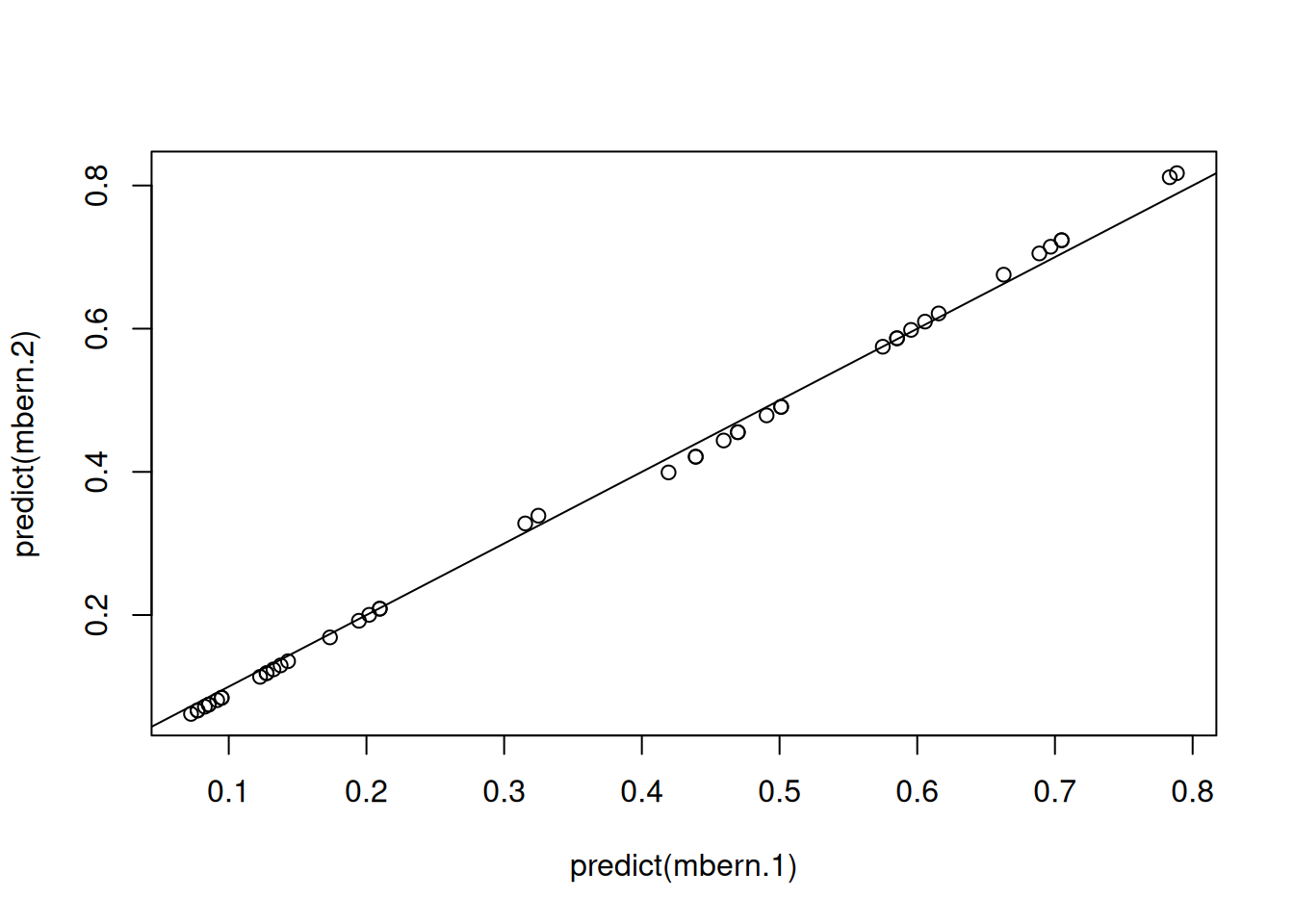
Figure 3.9: Predicted probabilities from a Bernoulli GLM from two models. The data and model structure are identical but in mbern.1 the residual variance was set to one and in mbern.2 the residual variance was set to three. The data provide no information about the residual variance.

We just have to be careful about how we express the results. Stating that the typehappy coefficient is -2.852 (the posterior mean estimate from mbern.1) is meaningless without putting it in the context of the assumed residual variance (one). Although the Diggle et al. (2004) approximation is less accurate than that in McCulloch and Searle (2001) we can use it rescale the estimates by the assumed residual variance (we’ll call it \(\sigma^{2}_{\texttt{units}}\)) in order to obtain the posterior distributions of the parameters under the assumption that the actual residual variance (we’ll call it \(\sigma^{2}_{e}\)) is equal to some other value. For location effects the posterior distribution needs to be multiplied by \(\sqrt{\frac{1+c^{2}\sigma^{2}_{e}}{1+c^{2}\sigma^{2}_{\texttt{units}}}}\) where \(c=16\sqrt{3}/15\pi\). If obtain estimates under the assumption that \(\sigma^{2}_{e}=0\) and we see the posterior distributions of the coefficients are very similar from the two models (Figure 3.10).

c2 <- ((16 * sqrt(3))/(15 * pi))^2
rescale.2 <- mbern.1$Sol * sqrt(1/(1 + c2 * 1))
rescale.3 <- mbern.2$Sol * sqrt(1/(1 + c2 * 3))
plot(mcmc.list(as.mcmc(rescale.2), as.mcmc(rescale.3)), density = FALSE)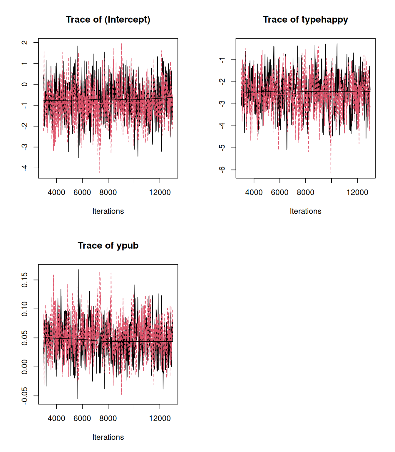

Figure 3.10: MCMC trace for rescaled coefficients of a Bernoulli GLM from two models (mbern.1 in black and mbern.2 in red). The data and model structure are identical but in mbern.1 the residual variance was set to one and in mbern.2 the residual variance was set to three. However, the coefficients have been rescaled using the Diggle et al. (2004) approximation such that they represent what the coefficients would be if the residual variance was zero. The data provide no information about the residual variance.

In addition, the posterior distributions are centred on the ML estimates obtained by glm which implicitly assumes \(\sigma^2_e=0\) (Figure 3.11).

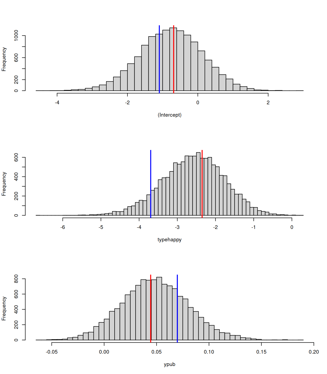
Figure 3.11: Posterior distributions for rescaled coefficients of a Bernoulli GLM (mbern.2). The rescaling gives approximate (but accurate) posterior distributions had the residual variance been set to zero, rather than three. The red lines indicate estimates from glm that implicitly assumes the residual variance is zero and the blue lines indicate the unscaled posterior means.

3.6.4 Probit link

The inverse-logit function is the cumulative distribution function for the logistic distribution. It makes sense that a cumulative distribution function for a continuous distribution that can take any value would serve as a good inverse link function for a probability: it takes any value between plus and minus infinity and squeezes it to be between zero and one. While the logit is the most common link function for binomial data, the probit link and complementary log-log (cloglog) link are also widely used. They are the cumulative distribution functions for the unit normal and standard Gumbel distributions respectively. In Figure 3.12 we can see how the probability changes as a function of a covariate (\(x\)) for the different links (with intercepts and slopes chosen so that the functions are matched at the origin).

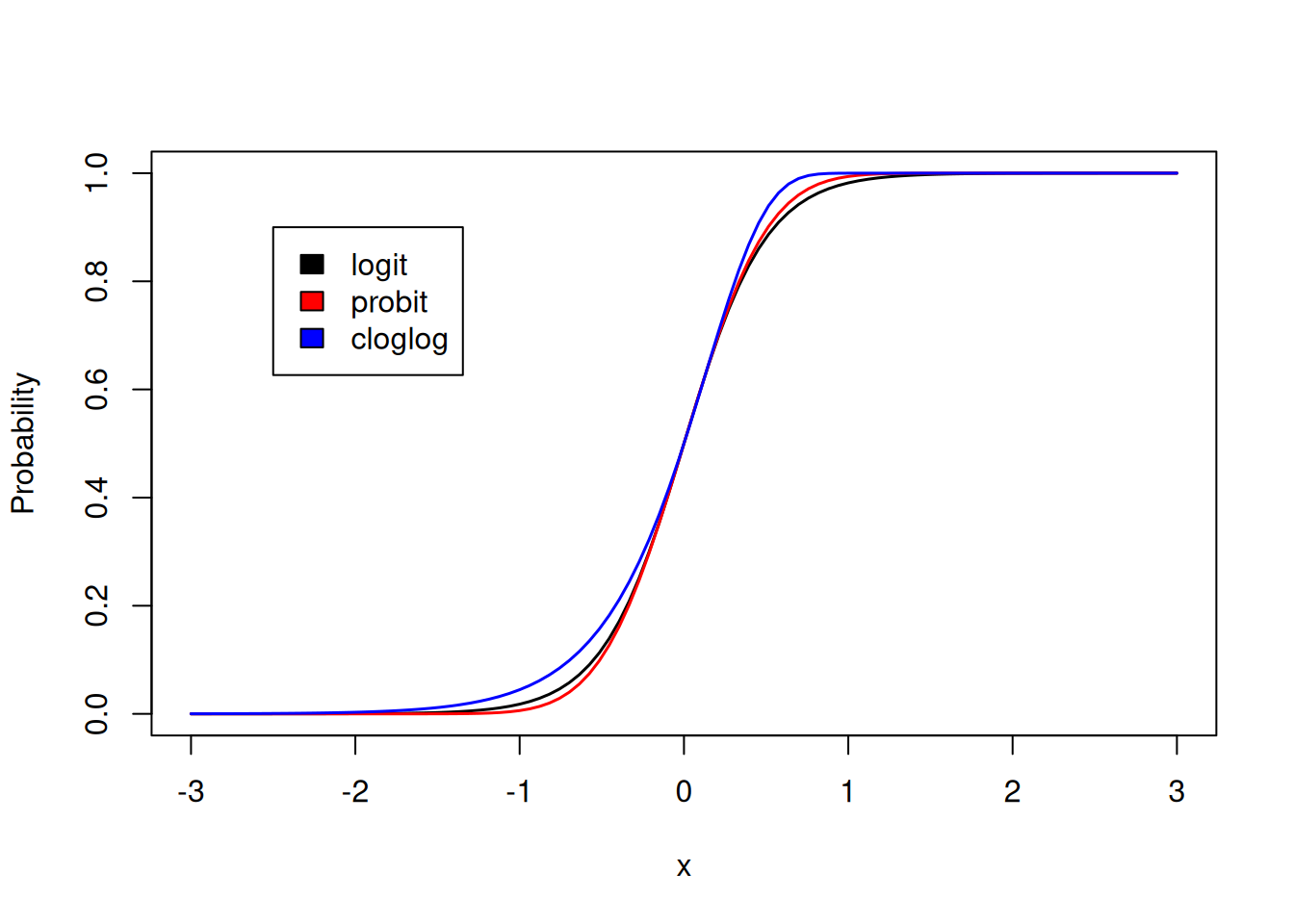
Figure 3.12: Predicted probabilities as a function of covariate \(x\) using the inverse logit (black), inverse probit (red) and inverse complementary log-log link functions. For each link the intercept and slope were chosen such that when \(x= 0\) the function equals 0.5 and has a derivative of one.

We can see that the link functions generate rather similar predicted probabilities, particularly the logit and probit links. For Bernoulli data, another way to conceptualise these link functions is in terms of threshold models. Imagine the case where we have managed to set the non-identifiable residual variance to zero and all residuals \(e\) are zero and can be omitted. The probability of success is then given by the inverse-link of \(\eta\). For probit link this would be the probability of getting a value less than \(\eta\) from the unit normal (the grey area in the left panel of Figure 3.13). Equivalently, it is the probability of getting a value greater than 0 from a normal with a mean equal to \(\eta\) and a standard deviation of one (the grey area in the right panel of Figure 3.13).

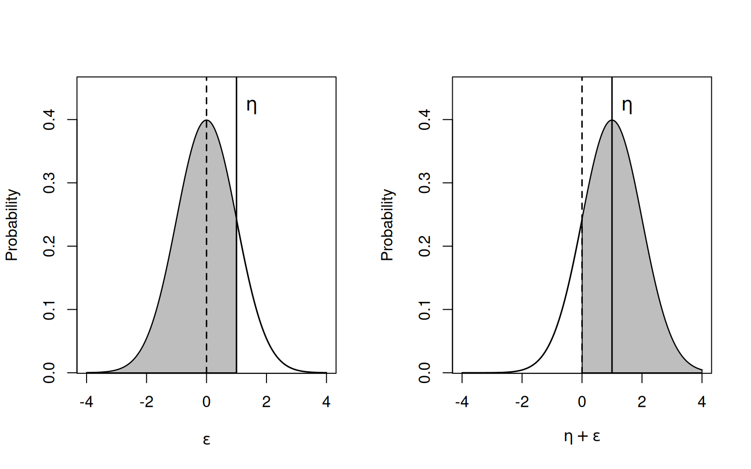
Figure 3.13: Probability density function for \(\epsilon\) (left) or \(\eta+\epsilon\) (right) where \(\epsilon\) is normal with mean zero and a standard deviation of one. Applying pnorm to \(\eta\) gives the shaded area on the left and is the probability of success using probit link. The shaded area on the right gives the same probability and is the chance of getting a value greater than zero from a normal with mean \(\eta\) and a standard deviation of one.

If we think explicitly about the normal deviates that underpin these probability calculations (we’ll call them \(\epsilon\)), then in the left panel \(\epsilon\) falls below the ‘threshold’ \(\eta\) with the required probability or in the right panel, \(\eta+\epsilon\) falls above the ‘threshold’ zero with the required probability. Since \(\epsilon\) is unit-normal we can equate \(\eta\) with \(e\) and \(\eta+\epsilon\) with \(l\) and apply the inverse link function \(\mathbf{1}_{\{l>0\}}\). This function outputs 1 (a success) if \(l>0\) and a failure otherwise (as in the right panel of Figure 3.13). This is implemented as family=threshold in MCMCglmm, and if the residual variance (i.e. the variance of \(\epsilon\) or \(e\)) is fixed at one corresponds exactly to standard probit regression⁹.

prior.mbinom.4 = list(R = list(V = 1, fix = 1))
mbinom.4 <- MCMCglmm(mean5 ~ type + ypub, family = "threshold", data = Grumpy, prior = prior.mbinom.4)

Unfortunately the same trick can’t be used for other link functions because the \(\epsilon\)’s’ cannot be equated with \(e\)’s because they come from different distributions. In some ways the probit link is a natural link function for models that contain random effects, which are also usually assumed to be normal. However, the downside is that the coefficients in a probit model do not have a direct interpretation like they do in a logit model. Nevertheless, both models give very similar predictions and are unlikely to be statistically distinguishable in the vast mean5 of cases (Figure 3.14).

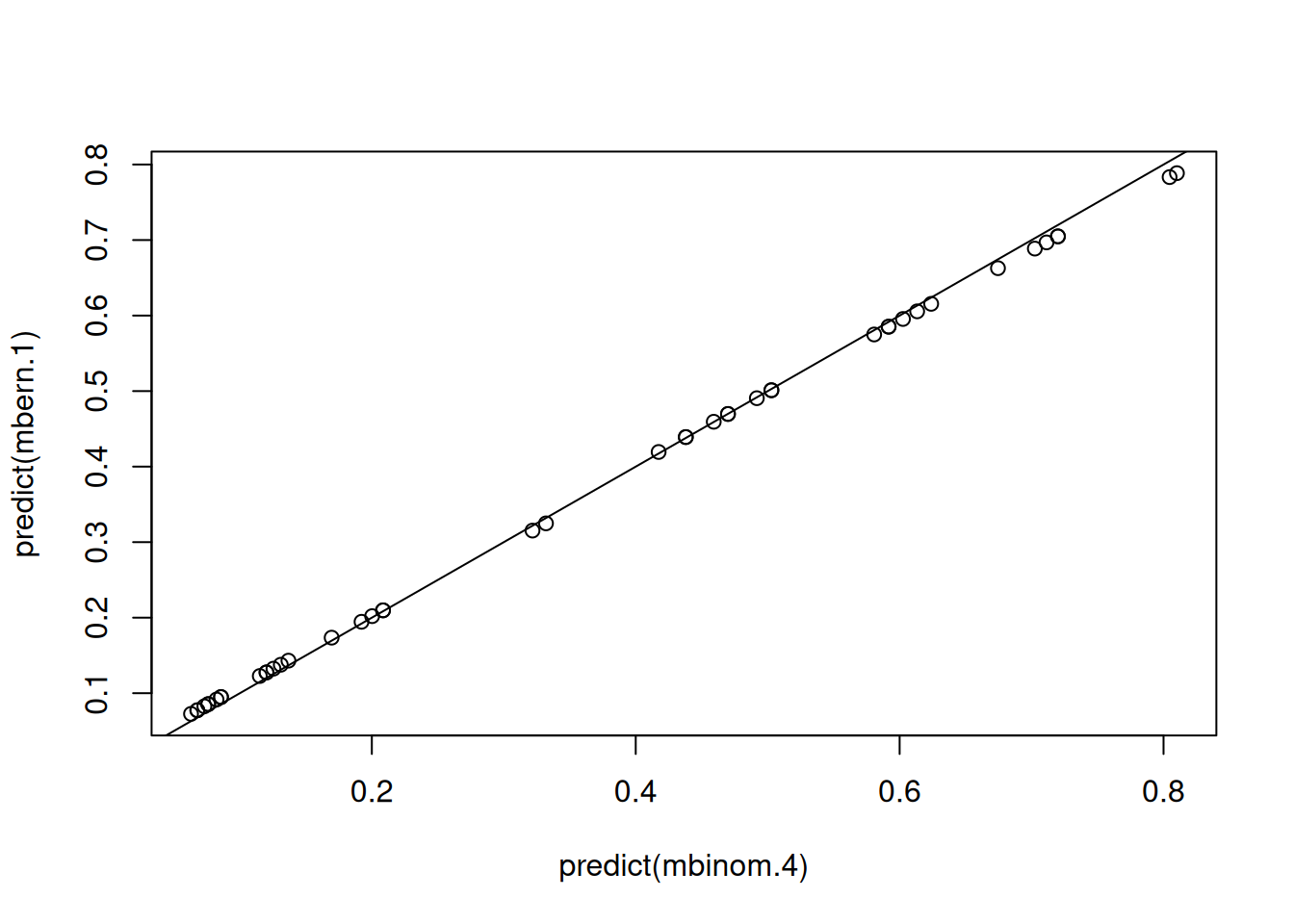
Figure 3.14: Predicted probabilities from a Bernoulli GLM from two models with the same model structure. However, mbern.1 uses a logit link with a residual variance set to one and in mbinom.4 uses a standard probit link.

3.7 Ordinal Data

Thinking about Bernoulli GLM’s in terms of thresholds provides a natural way of thinking about how we could model categorical data that falls into a natural ordering. For example, rather than dichotomising our outcome into those that had a mean score greater than, or less than, five, lets place the observations into three categories: (1, 4], (4, 6], (6, 10].

Grumpy$categories <- as.numeric(cut(Grumpy$y, c(1, 4, 6, 10)))

Rather than just having a single threshold at zero, we can imagine adding another threshold that chops the distribution of \(\eta+e=l\) into three regions, and hence probabilities. To make things simple we will just fit an intercept only model (so all observations have the same value of \(\eta\)) as this will be easier to visualise:

prior.mordinal = list(R = list(V = 1, fix = 1))
mordinal <- MCMCglmm(categories ~ 1, data = Grumpy, family = "threshold", prior = prior.mordinal)

The output of mordinal gives the intercept (\(\eta\) in this case) as before but also the additional threshold (cutpoint - stored as CP in the model object):

summary(mordinal)

## 
##  Iterations = 3001:12991
##  Thinning interval  = 10
##  Sample size  = 1000 
## 
##  DIC: 92.2748 
## 
##  R-structure:  ~units
## 
##       post.mean l-95% CI u-95% CI eff.samp
## units         1        1        1        0
## 
##  Location effects: categories ~ 1 
## 
##             post.mean l-95% CI u-95% CI eff.samp pMCMC  
## (Intercept)    0.4892   0.1356   0.9025      607 0.012 *
## ---
## Signif. codes:  0 '***' 0.001 '**' 0.01 '*' 0.05 '.' 0.1 ' ' 1
## 
##  Cutpoints: 
## 
##                            post.mean l-95% CI u-95% CI eff.samp
## cutpoint.traitcategories.1     1.322   0.8801    1.775    435.8

As we did in the right panel of Figure 3.13, we can draw this model with the estimated threshold (\(\gamma\)) included (Figure 3.15).

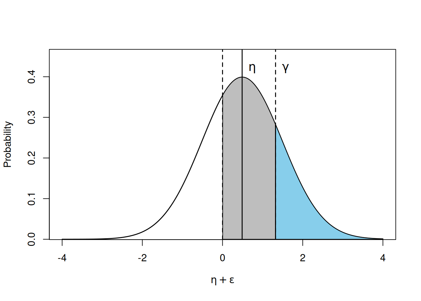
Figure 3.15: Probability density function for \(l=\eta+e\) where \(e\) is normal with mean zero and a standard deviation of one. \(\eta=\) 0.489 and was obtained from the model mordinal. The distribution is ‘cut’ into three regions by the fixed threshold at zero and the estimated threshold (\(\gamma\)) at 1.322. The shaded areas correspond to the probabilities of observing the three (ordered) outcomes.

The shaded areas give the probability for each category and the posterior mean probabilities can be easily calculated:

mean(pnorm(0, mordinal$Sol))

## [1] 0.3158146

mean(pnorm(mordinal$CP, mordinal$Sol) - pnorm(0, mordinal$Sol))

## [1] 0.4768311

mean(1 - pnorm(mordinal$CP, mordinal$Sol))

## [1] 0.2073543

These correspond closely to the observed frequencies in the data:

table(Grumpy$categories)/44

## 
##         1         2         3 
## 0.3181818 0.4772727 0.2045455

3.8 Non-zero Binomial Data

The final distribution that we will cover in this Chapter is something I have called the Non-zero Binomial which can be fitted using family="nzbinom". It was implemented for a specific application in which \(n\) (\(\texttt{number}\)) bumblebees were pooled and assayed for the presence of the Acute Bee Paralysis virus (Pascall et al. 2018). If the assay came back positive then at least one bee in the pool was infected and the outcome was recorded as a ‘success’ - otherwise non of the bees in the pool were infected and we have a ‘failure’ (\(\texttt{infected}\)).

data(ABPvirus)
ABPvirus[c(1:2, 98:99), ]

##        species number infected
## 1  B.pascuorum     10        0
## 2  B.pascuorum     10        0
## 98   B.lucorum      2        1
## 99   B.lucorum     10        0

The observations are essentially censored, and while we cover censoring more generally in Chapter 9, the Non-zero Binomial is perhaps best covered here. The probability of a success for the Non-zero Binomial (which we will designate as \(P\)) is \(1-(1-p)^n\) where \(p\) is the probability that an individual bumblebee was infected. If the number of bumblebees in a pool varies over observations, family="nzbinom" is a useful tool and the linear model is defined for the logit transform of \(p\), as in the standard binomial. In the standard Bernoulli model the residual variance could not be estimated and was fixed at some value. Perhaps surprisingly, there is some information to estimate the residual variance (overdispersion) in a Non-zero Binomial model as long as \(n\) varies over pools. However, the amount of information is so small that it is probably safest to fix the residual variance at some non-zero value (I use one as a convention) rather than risk sampling very high values of the residual variance that can cause numerical issues. We will ignore which species of bumblebee the observations were made on, as these are best treated as random effects (Chapter 4)

mnzbinom <- MCMCglmm(cbind(infected, number) ~ 1, family = "nzbinom", data = ABPvirus,
    prior = list(R = list(V = 1, fix = 1)))
summary(mnzbinom)

## 
##  Iterations = 3001:12991
##  Thinning interval  = 10
##  Sample size  = 1000 
## 
##  DIC: 131.4134 
## 
##  R-structure:  ~units
## 
##       post.mean l-95% CI u-95% CI eff.samp
## units         1        1        1        0
## 
##  Location effects: cbind(infected, number) ~ 1 
## 
##             post.mean l-95% CI u-95% CI eff.samp  pMCMC    
## (Intercept)    -3.088   -3.489   -2.656      510 <0.001 ***
## ---
## Signif. codes:  0 '***' 0.001 '**' 0.01 '*' 0.05 '.' 0.1 ' ' 1

The median probability of an individual bumblebee being infected is low: \(\texttt{plogis}(eta)=\) 0 such that the expected probability of at least one infection is small for the lowest pool-size (\(\texttt{number}=\) 2) and is still well below one in the largest pool size (\(\texttt{number}=\) 11) - see Figure 3.16.

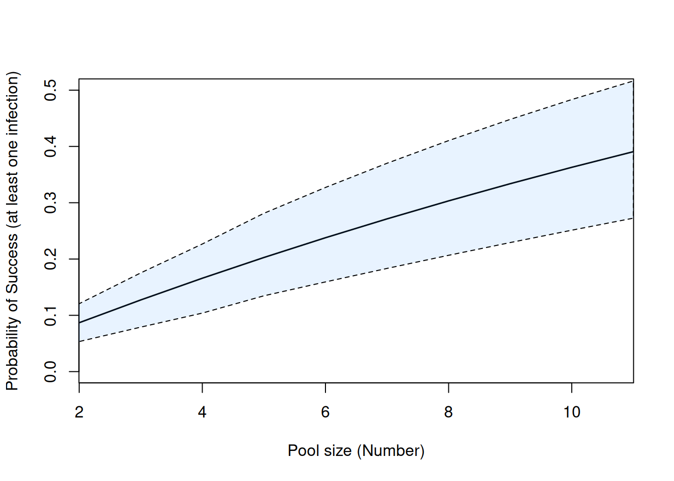
Figure 3.16: Probability of seeing at least one infection (\(P\)) in pools of varying size when the probability of an individual bumblebee being infected (\(p\)) is constant. The solid black line is the posterior mean and the shaded area is the 95% credible interval. The estimated median probability of an individual bumblebee being infected is0.044and the mean probability is0.044.

If the data set was larger and/or variation in the pool size was greater, there may be sufficient information to justify trying to estimate the residual variance, rather than fixing it to one. To see where the information comes from first imagine that you have information on samples all with a pool-size of 1. You could jut average you the resulting zeros and ones to get an estimate of \(P_1\) where the subscript designates the size of the pool for which the probability of at least one infection is calculated. Even if the probability of infection varied over individuals, the average probability \(E[p]\) is equal to \(P_1\), as we saw when we determined why variation in the probability cannot be estimated with standard Bernoulli data. Let’s then imagine we move to pool sizes of 2. \(P_2\) (the probability of at least one success in a pool of 2) is then \(E[1-(1-p)^2]\). If there is no variation in \(p\) then \(P_2=1-(1-P_1)^2\) since \(p\) is a constant and equal to \(P_1\). However, when there is variation in \(p\) the non-linearity in the function (i.e. \((1-p)^2\)) means that \(E[1-(1-p)^2]\) will deviate from \(1-(1-E[p])^2=1-(1-P_1)^2\): we expect the the number of successful pools of size 2 to be less than that predicted from estimating \(p\) from pools of size 1¹⁰. Consequently, the rate at which \(P\) asymptotes with increasing pool-size (as seen in Figure 3.16) provides information about how much variation in \(p\) exists.

3.9 Complete Separation

One potential issue that can occur in GLM is something known as complete separation or the extreme category problem. While it can occur for any distribution which is discrete, it is most commonly seen when the response is Bernoulli. It occurs when the predictors perfectly predict the outcome. For example, in Section 3.6.3 we generated Bernoulli data for each photo by assessing whether the mean score was greater than or less than five. Photo \(\texttt{type}\) is a very good predictor of the outcome, but not perfect:

table(mean5 = Grumpy$mean5, type = Grumpy$type)

##        type
## mean5   grumpy happy
##   FALSE      9    19
##   TRUE      13     3

However, if we removed the three observations for which the mean grumpy score was greater than five despite the person being happy, then \(\texttt{type}\) perfectly predicts the outcome. If we fit a probit model to these data, but using glm, a very strange thing happens:

data.cs <- subset(Grumpy, !(mean5 == TRUE & type == "happy"))

mcs <- glm(mean5 ~ type, family = binomial(link = probit), data = data.cs)
summary(mcs)

## 
## Call:
## glm(formula = mean5 ~ type, family = binomial(link = probit), 
##     data = data.cs)
## 
## Coefficients:
##             Estimate Std. Error z value Pr(>|z|)
## (Intercept)   0.2299     0.2698   0.852    0.394
## typehappy    -5.9798   359.8415  -0.017    0.987
## 
## (Dispersion parameter for binomial family taken to be 1)
## 
##     Null deviance: 51.221  on 40  degrees of freedom
## Residual deviance: 29.767  on 39  degrees of freedom
## AIC: 33.767
## 
## Number of Fisher Scoring iterations: 17

The coefficient for \(\texttt{typehappy}\) now has a huge standard error and the p-value is close to one, despite being a very good predictor of the outcome. This is known as the Hauck Jr and Donner (1977) effect. If we assess significance using Fisher’s exact test we get:

fisher.test(table(data.cs$mean5, data.cs$type))

## 
##  Fisher's Exact Test for Count Data
## 
## data:  table(data.cs$mean5, data.cs$type)
## p-value = 2.977e-05
## alternative hypothesis: true odds ratio is not equal to 1
## 95 percent confidence interval:
##  0.0000000 0.2098429
## sample estimates:
## odds ratio 
##          0

A very significant result, as expected.

The model fitted using \(\texttt{MCMCglmm}\) also behaves oddly with very poor mixing (Figure 3.17).

prior.mcs.2 = list(R = list(V = 1, fix = 1))
mcs.2 <- MCMCglmm(mean5 ~ type, family = "threshold", data = data.cs, prior = prior.mcs.2)
plot(mcs.2$Sol)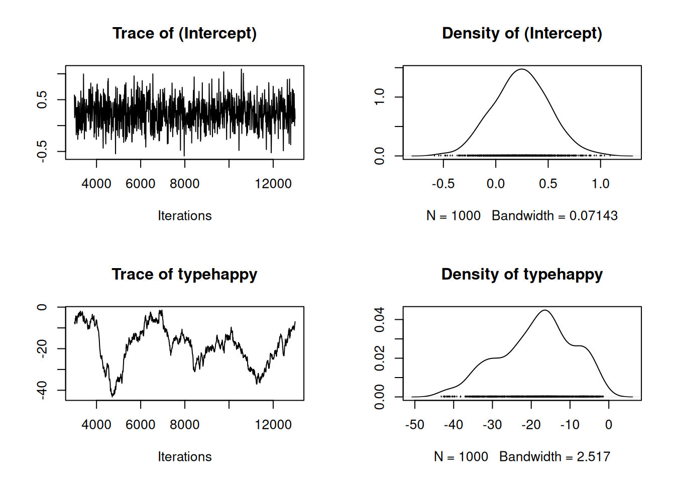

Figure 3.17: MCMC summary plots for the intercept and \(\texttt{typehappy}\) effect in a binary GLM (mcs.2) with probit link. For \(\texttt{happy}\) photos all 19 observations are failures (the mean grumpy score is less than 5) and we have complete separation. A normal prior with large variance was used for the model coefficients.

This strange behaviour occurs because the ML estimate for the probability of success is zero for \(\texttt{happy}\) photos. On the probit scale this translates into \(-\infty\) and so the ML estimate of the difference between \(\texttt{happy}\) and \(\texttt{grumpy}\) photos (the \(\texttt{typehappy}\) effect) will also be \(-\infty\). Consequently, with a flat prior on the \(\texttt{typehappy}\) effect the posterior distribution is improper. The default prior for model coefficients in \(\texttt{MCMCglmm}\) is not flat - they are normal with a large variance (\(10^8\)), but even so this diffuse prior can cause problems if there is complete (or near complete) separation. To see this, think about an intercept-only model. A diffuse prior on the probit scale puts a lot of density on very large positive or negative values and so puts a lot of density close to zero and one on the probability scale (see Figure 3.12). If the likelihood prevents the posterior from reaching these extremes then the prior has little influence because it is largely flat outside of the extremes (it is U-shaped). However, with complete separation the likelihood is indeed placing a lot of density at these extreme values and the prior holds the posterior at these values. If, on the other hand, we had specified the prior on the intercept to be normal with a mean of zero and a variance of one then the prior on the probability scale would be flat (since the inverse-link function is the cumulative density function for the unit normal). If a logit-link had been used then there is no normal prior that would result in flatness on the probability scale, and having a mean of zero and a variance of \(\pi^2/3\) (the variance of a logistic distribution) is a close as you can get if the residual variance had been zero (3.18).

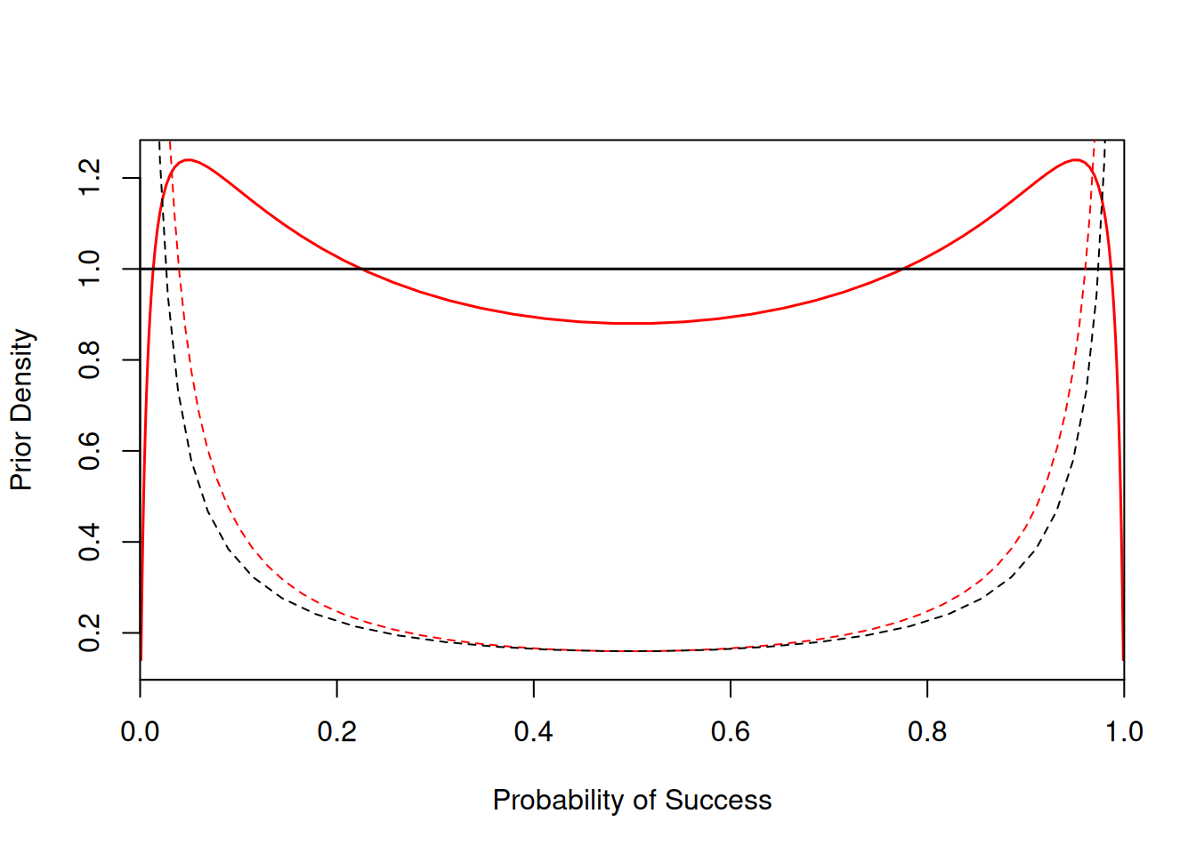
Figure 3.18: Prior density on the probability of success in an intercept-only Bernoulli GLM. The solid black line is for a standard probit link and a normal prior on the intercept with zero mean and a variance of one. The solid red line is for a standard logit link (with the residual variance set to zero) and a normal prior on the intercept with zero mean and a variance of one \(\pi^2/3\). The dashed lines are for when the variance is set to 100 (logit-link) or \(g^2 100\approx\) 39.3 (probit link) - see Section 3.9.1.

3.9.1 The Gelman, Jakulin, et al. (2008) prior

Ideally we would like to extend this idea so that we can define priors for coefficients associated with categorical and continuous predictors, not just the intercept. We would also like these priors to work well in the presence of variation caused by the addition of random effects (Chapter 4) and (depending on the family specified) a non-zero residual variance. What follows is very fiddly and a short summary and workflow can be found at the end.

For accommodating additional variance in the intercept-only model we can use a prior variance that is the sum of the link variance and the model-defined variance \(v\). In the Bernoulli models we’ve fitted \(v\) is just the residual variance which has been fixed at one. For the logit-link, the link variance is \(\pi^2/3\) which would result in a prior variance of \(1+\pi^2/3\). For the threshold link, the link variance is zero resulting in a prior variance of \(1\) (i.e. the standard probit where the residual variance is set to zero and the link variance is one). With random effects \(v\) may not be known a priori and a judicious choice about it’s magnitude would need to be made.

For models that contain predictors, Gelman, Jakulin, et al. (2008) suggested a prior for logit-link models where \(v=0\). They suggested that the input variables should be standardised prior to model fitting and that the the associated coefficients should have independent Cauchy priors with a scale of 10 for the (new) intercept and a scale of 2.5 for the remaining coefficients. The motivation behind this prior is that the average probability, defined by the new intercept, can have a wide range (\(10^{-9}\) \(-\) 1-\(10^{-9}\)). This is still rather U-shaped on the probability scale and in many applications a lower scale may perform better (Figure 3.18). The prior on the remaining coefficients imply that extremely large changes in probability between categorical predictors or per 0.5 standard deviations of a continuous predictor have low probability: for changes greater than ten on the logit scale, the prior density is 0.84. This combination of standardisation and prior naturally penalises higher order interactions, but it’s properties when random effects were fitted (or the residual variance was non-zero) were not explored.

Personally, I don’t like generic rescaling of inputs - I like my coefficients to have meaningful units. I would like to know how much my pot-belly is expected to grow per pistachio nut, not per standard deviation of pistachio nut consumption in the data set the dietician happened to have analysed. However, rather than standardising the inputs prior to model fitting we can fit them in their original form and place a prior on the coefficients that is equivalent to that recommended by Gelman, Jakulin, et al. (2008) had we rescaled the inputs. Although the Cauchy prior can probably be specified by treating the coefficients as random, here we will use a normal distribution with the same scales. This will penalise large coefficients more than the Cauchy prior.

To accommodate non-zero \(v\), we can multiply the scales recommended by Gelman, Jakulin, et al. (2008) by \(\sqrt{1/(1+c^2\texttt{v})}\) such that the same prior interpretation can be given (approximately) to the marginal effects of the predictors (see earlier). A change of one logit is neither equivalent or proportional to a change of one probit. For example, going from -1 to -2 on the logit scale we move from a probability of 0.27 to 0.12 but on the probit scale a change from -1 to -2 results in a change of probability from 0.16 to 0.02. Around zero (i.e a probability of 0.5 in both cases) the change in probability per logit is 0.25 and the change in probability per probit is 0.399. Consequently, we can multiply the scales recommended by Gelman, Jakulin, et al. (2008) by \(g=\) 0.25 / 0.399=dlogis(0)/dnorm(0)=\(\sqrt{2\pi}/4\) to achieve approximate equivalence. Note this was done when determining the regression coefficients to produce Figure 3.12 and the two prior densities diverge as the probability moves away from 0.5 (see Figure 3.18 also). When additional variance is present we can multiply the original scales by \(\sqrt{g^2/\texttt{v}}\) when family="threshold" is used.

The function gelman.prior takes the (fixed effect) model formula as its first argument and together with the data.frame the model is to be fitted to (passed in the argument data) generates the prior specification (\(\texttt{mu}\) and \(\texttt{V}\)) for the model parameters, had the inputs been scaled as in Gelman, Jakulin, et al. (2008). The argument intercept.scale specifies the scale of the normal (standard deviation) for the intercept and the argument coef.scale specifies the scale of the normal for the remaining parameters - both defined as if inputs were scaled¹¹. By default these scales are set to one.

This is all quite confusing and here are the main points and a practical workflow.

1. Gelman, Jakulin, et al. (2008) recommended standardising inputs prior to logistic regression and using a prior that allows a wide range for the average probability of success but penalises large effects associated with predictors.

2. The function gelman.prior helps set up a prior similar to that recommended by Gelman, Jakulin, et al. (2008) but a) using a normal in place of a Cauchy and b) not requiring the inputs to be standardised prior to analysis.

3. To gelman.prior you should pass your model formula (fixed in MCMCglmm) and data that will be used in the analysis.

4. You also need to decide on a prior scale for the mean (intercept.scale) and the coefficients of the standardised inputs (coef.scale). To achieve a prior as close to that recommended by Gelman, Jakulin, et al. (2008) you can use \(10\sqrt{1/(1+c^2\texttt{v})}\) (family="binomial") or \(10\sqrt{g^2/\texttt{v}}\) (family="threshold") for intercept.scale and \(2.5\sqrt{1/(1+c^2\texttt{v})}\) (family="binomial") or \(2.5\sqrt{g^2/\texttt{v}}\) (family="threshold") for coef.scale. \(c=16\sqrt{3}/15\pi\) and g=\(\sqrt{2\pi}/4.\)

5. The output of gelman.prior can be passed directly as the fixed effect prior (i.e. prior=list(B=gelman.prior(...)).

We can try this out for the model we fitted to the data set with complete separation:

g <- sqrt(2 * pi)/4

prior.mcs.3 = list(B = gelman.prior(~type, data = data.cs, coef.scale = g * 2.5,
    intercept.scale = g * 10), R = list(V = 1, fix = 1))

mcs.3 <- MCMCglmm(mean5 ~ type, family = "threshold", data = data.cs, prior = prior.mcs.3)
plot(mcs.3$Sol)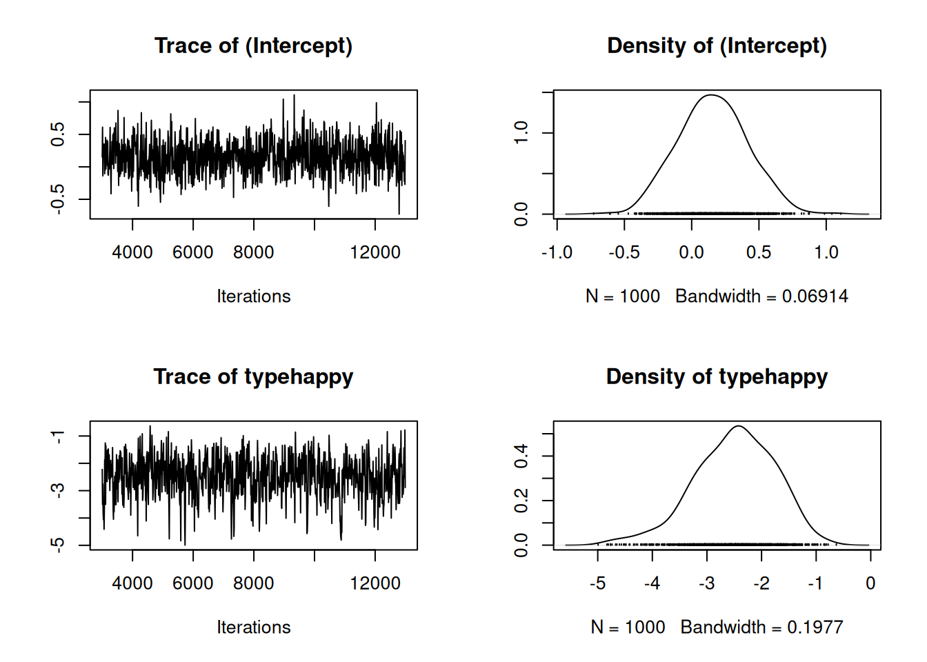

Figure 3.19: MCMC summary plots for the intercept and \(\texttt{type}\) effect in a binary GLM (mcs.3) with probit link. For \(\texttt{happy}\) photos all 19 observations are failures (the mean grumpy score is less than 5) and we have complete separation. A prior was set up using gelman.prior that penalises very large differences between \(\texttt{happy}\) and \(\texttt{grumpy}\) photos.

and we can see that the chain now looks well behaved (Figure 3.19). We can calculate the posterior distribution for the probability of success for \(\texttt{happy}\) photos, where we had complete separation (19 failures and 0 successes). If we compare this posterior distribution with that from the model that used the diffuse (default) prior, we can see that all the density is not concentrated at very low density 3.20. This seems reasonable given that zero successes and 19 failures has a reasonable probability (0.135)even when the probability of success is 0.1.

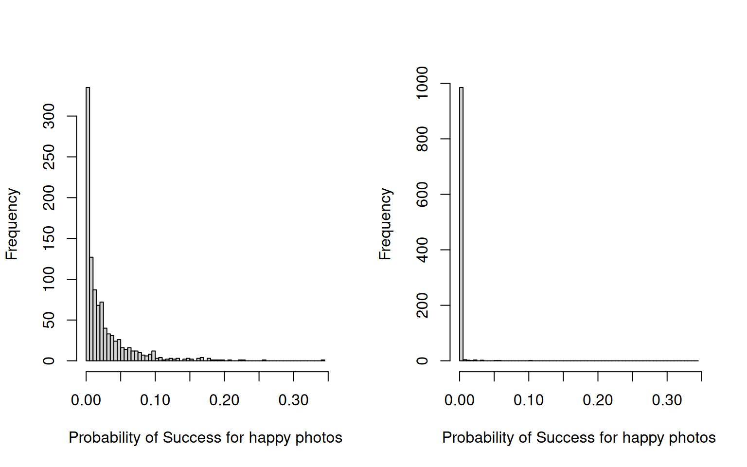
Figure 3.20: Posterior distribution for the probability of success for \(\texttt{happy}\) photos, where there was complete separation (19 failures and 0 successes). For model mcs.3 (left) a prior was set up using gelman.prior that penalised large differences between \(\texttt{happy}\) and \(\texttt{grumpy}\) photos. For model mcs.2 (right) the default diffuse prior was used.

References

Albert, James H, and Siddhartha Chib. 1993. “Bayesian Analysis of Binary and Polychotomous Response Data.” Journal of the American Statistical Association 88 (422): 669–79.

Diggle, P., P. Heagerty, K. Liang, and S. Zeger. 2004. Analysis of Longitudinal Data. II. Oxford University Press.

Gelman, A., A. Jakulin, M. G. Pittau, and Y. Su. 2008. “A Weakly Informative Default Prior Distribution for Logistic and Other Regression Models.”

Hauck Jr, Walter W, and Allan Donner. 1977. “Wald’s Test as Applied to Hypotheses in Logit Analysis.” Journal of the American Statistical Association 72 (360a): 851–53.

Hinde, John. 1982. “Compound Poisson Regression Models.” In Glim 82: Proceedings of the International Conference on Generalised Linear Models, 109–21. Springer.

McCulloch, C. E., and S. R. Searle. 2001. Generalized, Linear and Mixed Models. Wiley Series in Probability and Statistics. New York: John Wiley & Sons.

Pascall, David J, Matthew C Tinsley, Darren J Obbard, and Lena Wilfert. 2018. “Host Evolutionary History Predicts Virus Prevalence Across Bumblebee Species.” BioRxiv, 498717.

---

4. This is a bit disingenuous. The MCMC algorithm implemented in depends on a non-zero residual variance to ensure mixing - if the residual variance was set to zero (i.e. no overdispersion in GLM(M)) then the Markov chain would be reducible.↩︎

5. Since the residuals are assumed normal the exponentiated residuals are log-normal, and so this model is often referred to as the Poisson log-normal (Hinde 1982). The Negative Binomial distribution is a commonly used alternative for overdispersed count data. The Negative Binomial is conceptually identical to the Poisson log-normal except the exponentiated residuals are assumed to be gamma distributed. The log-normal and gamma distributions are so similar that for most data sets it would be hard to distinguish between the Negative Binomial and the Poisson log-normal.↩︎

6. In versions <4.0 family=“binomial” was not an option. family="categorical" had to be used with Bernoulli data passed as a single column of success/failure and family="multinomial2" had to be used with Binomial data passed as two columns of successes and failures. In multi-response models (Chapter 7) “categorical” and “multinomial2” should be used respectively.↩︎

7. When \(x\) is small \(\textrm{exp}(x)\approx 1+x\).↩︎

8. For more complicated models a (co)variance matrix may be estimated for a particular random component rather than just a single variance as here. In such cases, V is a matrix. The value at which (part of) the (co)variance matrix is fixed at is determined by V. Any elements of the covariance matrix in rows and/or columns equal to or greater than fix are fixed. In the case of a single variance fix=1 simply fixes the variance (element 1,1 of the (co)variance matrix) at whatever is specified in V (one in this example).↩︎

9. We saw that with Bernoulli variables the \(\texttt{units}\) variance is not identifiable and needs to be fixed at some value. If the \(\texttt{units}\) variance is set to one when using family="threshold" we end up with the standard probit link. Wen exploring the logit link, we saw how we could take estimates of the location effects and variances from a model with some specified \(\texttt{units}\) variance and obtain what those estimates would be had we assumed some other value for the \(\texttt{units}\) variance, at least approximately. For family="threshold" this can be done exactly: location effects can be scaled by \(\sqrt{\frac{1+\sigma^2_e}{1+\sigma^2_\texttt{units}}}\) and variances by \(\frac{1+\sigma^2_e}{1+\sigma^2_\texttt{units}}\) to obtain estimates had the units variance been set to \(\sigma^2_e\) rather than \(\sigma^2_\texttt{units}\). family="ordinal" is also available in \(\texttt{MCMCglmm}\) but it is only retained to ensure back compatibility: it is equivalent to family="threshold" with the variance fixed at the specified value plus one. Consequently, it can be considered as a reprameterised version of family="threshold". When family="ordinal" was implemented I had misunderstood the paper by Albert and Chib (1993) and didn’t realise the latent variable could be Gibbs sampled with a threshold link (\(\mathbf{1}_{\{l>0\}}\)).↩︎

10. I know that \(E[1-(1-p)^2]\) will be less than \(1-(1-E[p])^2\) because of Jensen’s inequality. Jensen’s inequality tells us that \(E[f(x)]\) will be less than \(f(E[x])\) if \(f\) is convex, or greater than than \(f(E[x])\) if \(f\) is concave. In the current example, \(f(x) = (1-x)^2=1-2x+x^2\), which is a quadratic with a positive quadratic coefficient and so convex.↩︎

11. In MCMCglmm versions <3.0, gelman.prior took the arguments scale and intercept instead of coef.scale and coef.intercept. In addition the old version only returned the prior covariance matrix but now passes a list with the prior means (mu) and the prior covariance matrix (V).↩︎