2 Bayesian Analysis and MCMC

In this Chapter I cover the basics of Bayesian analysis and Markov chain Monte Carlo (MCMC) techniques. Exposure to these ideas, and statistics in general, has increased dramatically since these notes were first written. Many readers may therefore wish to skip straight to later chapters that cover \(\texttt{MCMCglmm}\) more specifically.

2.1 Introduction

There are fundamental differences between frequentist and Bayesian approaches, but for those of us interested in applied statistics the hope is that these differences do not translate into practical differences, and this is often the case. My advice would be if you can fit the same model using different packages and/or methods do so, and if they give very different answers worry. In some cases differences will exist, and it is important to know why, and which method is more appropriate for the data in hand.

In the context of a generalised linear mixed model (GLMM), here are what I see as the pro’s and cons of using (restricted) maximum likelihood (REML) versus Bayesian MCMC methods. REML is fast and easy to use, whereas MCMC can be slow and technically more challenging. Particularly challenging is the specification of a sensible prior, something which is a non-issue in a REML analysis. However, analytical results for non-Gaussian GLMM are generally not available, and REML based procedures use approximate likelihood methods that may not work well. MCMC is also an approximation but the accuracy of the approximation increases the longer the analysis is run for, being exact at the limit. In addition, REML uses large-sample theory to derive approximate confidence intervals that may have very poor coverage, especially for variance components. Again, MCMC measures of confidence are exact, up to Monte Carlo error, and provide an easy and intuitive way of obtaining measures of confidence on derived statistics such as ratios of variances, correlations and predictions.

To illustrate the differences between the approaches let’s imagine we’ve observed several draws (stored in the vector \({\bf y}\)) from a standard normal (i.e. \(\mu=0\) and \(\sigma^{2}=1\)). The likelihood is the probability of the data given the parameters:

\[Pr({\bf y} | \mu, \sigma^{2})\]

This is a conditional distribution, where the conditioning is on the model parameters which are taken as fixed and known. In a way this is quite odd because we’ve already observed the data, and we don’t know what the parameter values are. In a Bayesian analysis we evaluate the conditional probability of the model parameters given the observed data:

\[Pr(\mu, \sigma^{2} | {\bf y}) \label{post1-eq} \tag{2.1}\]

which seems more reasonable, until we realise that this probability is proportional to

\[Pr({\bf y} | \mu, \sigma^{2})Pr(\mu, \sigma^{2})\]

where the first term is the likelihood, and the second term represents our prior belief in the values that the model parameters could take. Because the choice of prior is rarely justified by an objective quantification of the state of knowledge it has come under criticism, and indeed we will see later that the choice of prior can make a difference.

2.2 Likelihood

We can generate 5 observations from this distribution using rnorm:

Ndata <- data.frame(y = rnorm(5, mean = 0, sd = 1))
Ndata$y

## [1] -1.01500872 -0.07963674 -0.23298702 -0.81726793  0.77209084

We can plot the probability density function for the standard normal using dnorm and we can then place the 5 data on it:

possible.y<-seq(-3,3,0.1)                    # possible values of y
Probability<-dnorm(possible.y, mean=0, sd=1) # density of possible values 
plot(Probability~possible.y, type="l", ylab="Density", xlab="y")
Probability.y<-dnorm(Ndata$y, mean=0, sd=1)  # density of actual values
points(Probability.y~Ndata$y)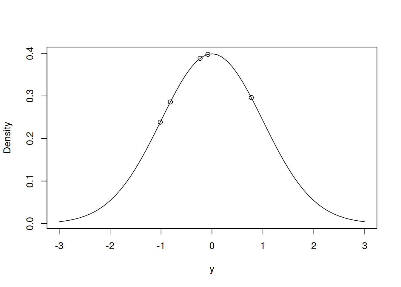

Figure 2.1: Probability density function for the unit normal with the data points overlaid

The likelihood of these data, conditioning on \(\mu=0\) and \(\sigma^2=1\), is proportional to the product of the densities (read off the y-axis on Figure 2.1):

prod(dnorm(Ndata$y, mean = 0, sd = 1))

## [1] 0.003113051

Of course we don’t know the true mean and variance and so we may want to ask how probable the data would be if, say, \(\mu=0\), and \(\sigma^2=0.5\):

prod(dnorm(Ndata$y, mean = 0, sd = sqrt(0.5)))

## [1] 0.005424967

It would seem that the data are more likely under this set of parameters than the true parameters, which we must expect some of the time just from random sampling. To get some idea as to why this might be the case we can overlay the two densities (Figure 2.2), and we can see that although some data points (e.g. -1.015) are more likely with the true parameters, in aggregate the new parameters produce a higher likelihood.

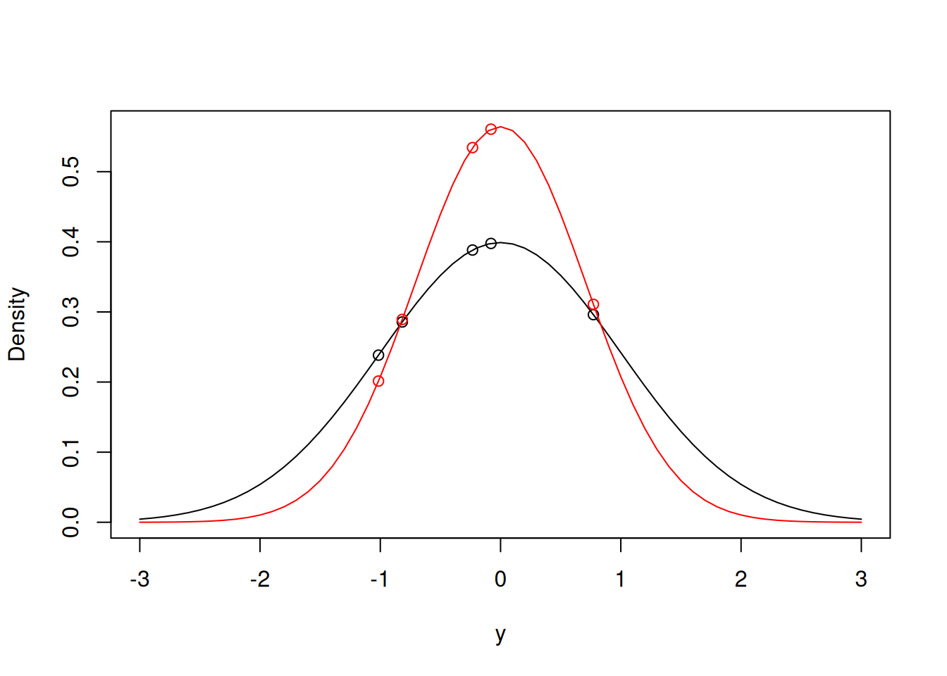
Figure 2.2: Two probability density functions for normal distributions with means of zero, and a variance of one (black line) and a variance of 0.5 (red line). The data points are overlaid.

The likelihood of the data can be calculated on a grid of possible parameter values to produce a likelihood surface, as in Figure 2.3. The densities on the contours have been scaled so they are relative to the density of the parameter values that have the highest density (the maximum likelihood estimate of the two parameters). Two things are apparent. First, although the surface is symmetric about the line \(\mu = \hat{\mu}\) (where \(\hat{}\) stands for maximum likelihood estimate) the surface is far from symmetric about the line \(\sigma^{2} = \hat{\sigma}^{2}\). Second, there are a large range of parameter values for which the data are only 10 times less likely than if the data were generated under the maximum likelihood estimates.

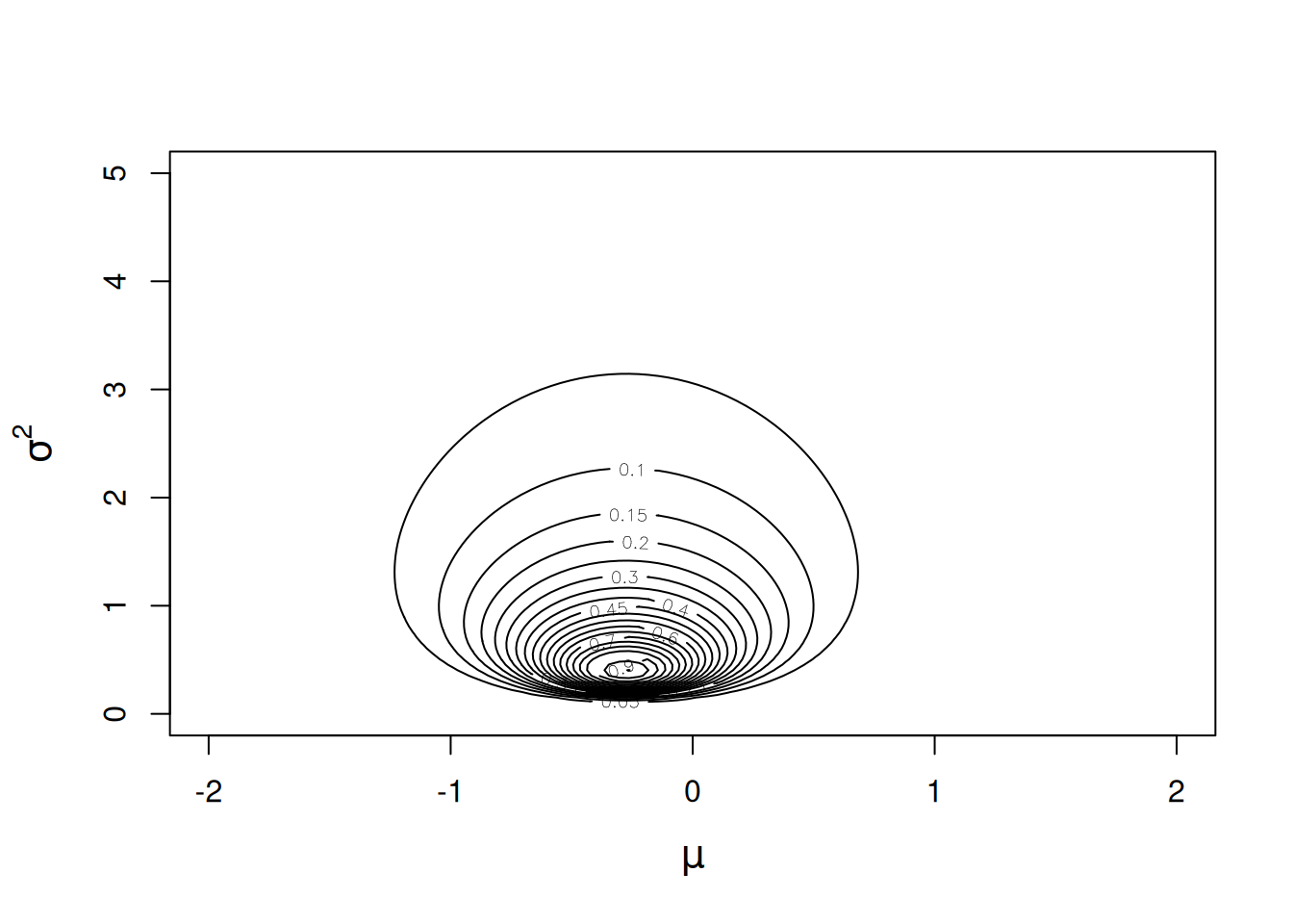
Figure 2.3: Likelihood surface for the likelihood \(Pr({\bf y}|\mu, \sigma^{2})\). The likelihood has been normalised so that the maximum likelihood has a value of one.

2.2.1 Maximum Likelihood (ML)

The ML estimator is the combination of \(\mu\) and \(\sigma^{2}\) that make the data most likely. Although we could evaluate the density on a grid of parameter values (as we did to produce Figure 2.3) in order to locate the maximum, for such a simple problem the ML estimator can be derived analytically. However, so we don’t have to meet some nasty maths later, I’ll introduce and use one of R’s generic optimising routines that can be used to maximise the likelihood function (in practice, the log-likelihood is maximised to avoid numerical problems):

lik <- function(par, y, log = FALSE) {
    if (log) {
        l <- sum(dnorm(y, mean = par[1], sd = sqrt(par[2]), log = TRUE))
    } else {
        l <- prod(dnorm(y, mean = par[1], sd = sqrt(par[2])))
    }
    return(l)
}
# function which takes the parameter vector (mean and *variance*) and the data
# and returns the (log) likelihood

MLest <- optim(c(mean = 0, var = 1), fn = lik, y = Ndata$y, log = TRUE, control = list(fnscale = -1,
    reltol = 1e-16))$par

The first call to optim are starting values for the optimisation algorithm, and the second argument (fn) is the function to be maximised. By default optim will try to minimise the function hence multiplying by -1 (fnscale = -1). The algorithm has successfully found the mode:

MLest

##       mean        var 
## -0.2745619  0.3955995

Alternatively we could also fit the model using glm, which by default assumes the response is normal:

m1a.1 <- glm(y ~ 1, data = Ndata)
summary(m1a.1)

## 
## Call:
## glm(formula = y ~ 1, data = Ndata)
## 
## Coefficients:
##             Estimate Std. Error t value Pr(>|t|)
## (Intercept)  -0.2746     0.3145  -0.873    0.432
## 
## (Dispersion parameter for gaussian family taken to be 0.4944994)
## 
##     Null deviance: 1.978  on 4  degrees of freedom
## Residual deviance: 1.978  on 4  degrees of freedom
## AIC: 13.553
## 
## Number of Fisher Scoring iterations: 2

Here we see that although the estimate of the mean (intercept) is the same, the estimate of the variance (the dispersion parameter: 0.494) is higher when fitting the model using glm. In fact the ML estimate is a factor \(\frac{n}{n-1}\) smaller because the glm estimate has used Bessel’s correction:

MLest["var"] * (5/4)

##       var 
## 0.4944994

2.2.2 Restricted Maximum Likelihood (REML)

Why do we use Bessel’s correction? Imagine we had only observed the first two values of \({\bf y}\) (Figure 2.4). The variance is defined as the average squared distance between a random variable and the true mean. However, the ML estimator of the variance is the average squared distance between the random variable and the ML estimate of the mean. Since the ML estimator of the mean is the average of the two numbers (the dashed line) then the average squared distance will always be smaller than if the true mean was used, unless the ML estimate of the mean and the true mean coincide. This is why we use Bessel’s \(n-1\) correction when estimating the variance from the sum of squares, or why we divide by \(n-n_p\) when estimating the residual variance in a liner model with \(n_p\) parameters, or more generally why we use REML in linear mixed models. Why these corrections for uncertainty in the mean, or model parameters, have this form can be understood from a Bayesian perspective (see Section 2.6).

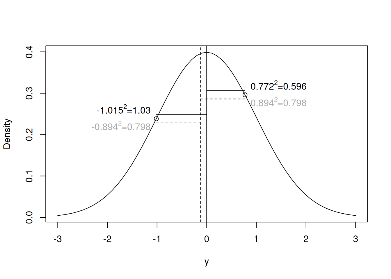
Figure 2.4: Probability density function for the unit normal with two realisations overlaid. The solid vertical line is the true mean, whereas the vertical dashed line is the mean of the two realisations (the ML estimator of the mean). The variance is the expected squared distance between the true mean and the realisations. The ML estimator of the variance is the average squared distance between the ML mean and the realisations (horizontal dashed lines), which is always smaller than the average squared distance between the true mean and the realisations (horizontal solid lines)

2.3 Prior Distribution

\(\texttt{MCMCglmm}\) uses a normal prior for the fixed effects and an inverse-Wishart prior for the residual variance. In the current model their is a single fixed effect (\(\mu\)) and a scalar (residual) variance (\(\sigma^2\)). For the mean we will use the default prior - a diffuse normal centred around zero but with very large variance (\(10^{8}\)). For the residual variance, the inverse-Wishart prior takes two scalar parameters. In \(\texttt{MCMCglmm}\) this is parameterised through the parameters \(\texttt{V}\) and \(\texttt{nu}\). The distribution tends to a point mass on \(\texttt{V}\) as the degree of belief parameter, \(\texttt{nu}\) goes to infinity. We will defer a full discussion of the inverse-Wishart prior to Section 2.6 and for now we will use the prior specification \(\texttt{V}=1\) and \(\texttt{nu}=0.002\) which used to be frequently used for variances. The function dprior can be used to obtain the prior density for a variance (or standard deviation) given a \(\texttt{MCMCglmm}\) specification and we can plot this in order to visualise what the distribution looks like (Figure 2.5).

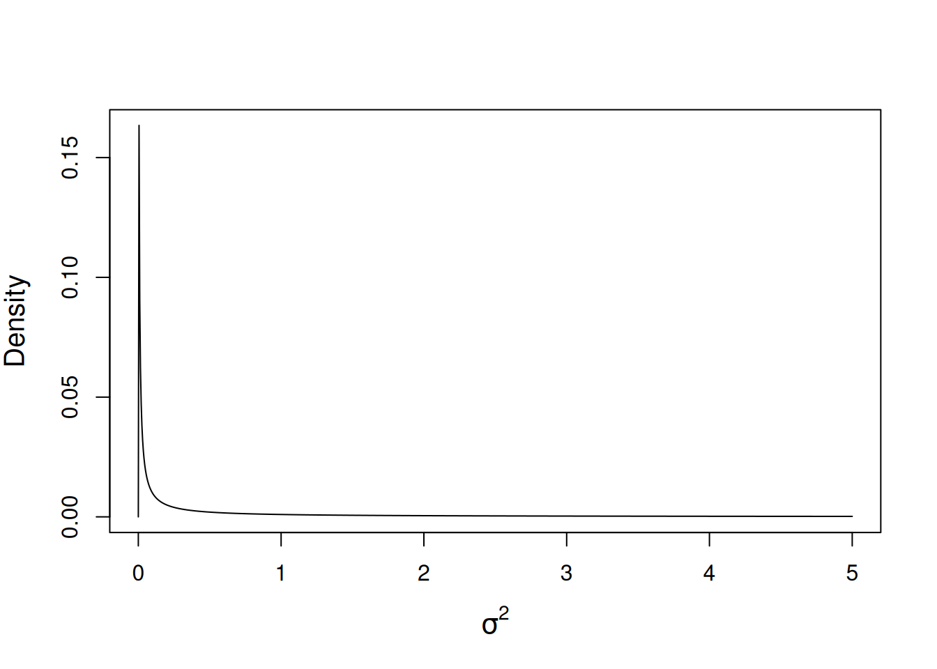
Figure 2.5: Probability density function for a univariate inverse-Wishart with the variance at the limit set to 1 (\(\texttt{V}=1\)) and a degree of belief parameter set to 0.002 (\(\texttt{nu}=0.002\)).

As before we can write a function for calculating the (log) prior probability:

prior.p <- function(par, priorB, priorR, log = FALSE) {
    if (log) {
        d <- dnorm(par[1], mean = priorB$mu, sd = sqrt(priorB$V), log = TRUE) + dprior(par[2],
            priorR, log = TRUE)
    } else {
        d <- dnorm(par[1], mean = priorB$mu, sd = sqrt(priorB$V)) * dprior(par[2],
            priorR)
    }
    return(d)
}

where priorR is a list with elements V and nu specifying the prior for the variance, and priorB is a list with elements mu and V specifying the prior for the mean. \(\texttt{MCMCglmm}\) takes these prior specifications as a list:

prior <- list(R = list(V = 1, nu = 0.002), B = list(mu = 0, V = 1e+08))

2.4 Posterior Distribution

By multiplying the likelihood by the prior probability for that set of parameters we can get the posterior probability up to a proportional constant. We can write a function for doing this:

likprior <- function(par, y, priorB, priorR, log = FALSE) {

    if (log) {
        pd <- lik(par, y, log = TRUE) + prior.p(par, priorB = priorB, priorR = priorR,
            log = TRUE)
    } else {
        pd <- lik(par, y) * prior.p(par, priorB = priorB, priorR = priorR)
    }
    return(pd)
}

and we can overlay the posterior density (scaled by the posterior density at the posterior mode) on the likelihood surface we calculated before (Figure 2.3).

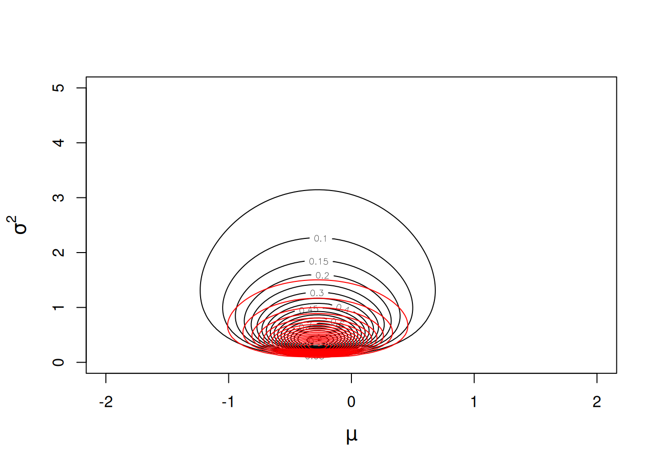
Figure 2.6: Likelihood surface for the likelihood \(Pr({\bf y}|\mu, \sigma^{2})\) in black, and the posterior distribution \(Pr(\mu, \sigma^{2} | {\bf y})\) in red. The likelihood has been normalised so that the maximum likelihood has a value of one, and the posterior distribution has been normalised so that the posterior mode has a value of one. The prior distributions \(Pr(\mu)\sim N(0, 10^8)\) and \(Pr(\sigma^{2})\sim IW(\texttt{V}=1, \texttt{nu}=0.002)\) were used.

The prior has some influence on the posterior mode of the variance, and we can use an optimisation algorithm again to locate the mode:

Best <- optim(c(mean = 0, var = 1), fn = likprior, y = Ndata$y, priorB = prior$B,
    priorR = prior$R, log = TRUE, method = "L-BFGS-B", lower = c(-1e+05, 1e-05),
    upper = c(1e+05, 1e+05), control = list(fnscale = -1, factr = 1e-16))$par
Best

##       mean        var 
## -0.2745613  0.2827783

The posterior mode for the mean is essentially identical to the ML estimate, but the posterior mode for the variance is even less than the ML estimate, which is known to be downwardly biased. The reason that the ML estimate is downwardly biased is because it did not take into account the uncertainty in the mean, as we saw when discussing the motivation behind REML. In a Bayesian analysis we can do this by evaluating the marginal distribution of \(\sigma^{2}\) by averaging over the uncertainty in the mean. Before we do this, however, it will be instructive to see why this would be hard using our function that simply multiplies the likelihood by the prior (likprior). This function (the probabilities on the right-hand side) is only proprtional to the posterior density (the left-hand side), not equal to it, implying

\[Pr(\mu, \sigma^{2} | {\bf y}) = \frac{1}{C} Pr({\bf y} | \mu, \sigma^{2})Pr(\mu, \sigma^{2})\]

where \(C\) is some constant. In some cases this is not an issue - when finding the posterior mode it was not an issue since the parameters that maximise the posterior density would also maximise the posterior density scaled by \(C\). Similarly, if we wanted to make relative statements about posterior probabilities, then \(C\) would cancel. For example, we can see how much more likely a variance of a half is versus a variance of one (assuming the mean is zero):

p.0.5 <- likprior(c(0, 0.5), y = Ndata$y, priorB = prior$B, priorR = prior$R)
p.1.0 <- likprior(c(0, 1), y = Ndata$y, priorB = prior$B, priorR = prior$R)

p.0.5/p.1.0

## [1] 3.484236

However, in many instances we would like to work with the normalised posterior density, so how do we get \(C\)? Well we know that if we took the posterior probability of being any combination of \(\mu\) and \(\sigma^{2}\) it must be equal to one:

\[\int_{\sigma^2}\int_\mu Pr(\mu, \sigma^{2} | {\bf y})d\mu d\sigma^2=1\]

and so because

\[1 =\frac{1}{C}\int_{\sigma^2}\int_\mu Pr({\bf y} | \mu, \sigma^{2})Pr(\mu, \sigma^{2})d\mu d\sigma^2\]

we can integrate our parameters over likprior to get \(C\). Not easy, and requires numerical integration:

C <- adaptIntegrate(likprior, y = Ndata$y, priorR = prior$R, priorB = prior$B, lower = c(-Inf,
    0), upper = c(Inf, Inf))$integral

The posterior density for \(\mu=0\) and \(\sigma^2=0.5\) is p.0.5/C=0.937. Neither interesting or particularly interpretable, and often we want to perform additional integration in order to compute quantities of interest. For example, imagine we wanted to know the probability that the parameters lay in the region of parameter space we were plotting, i.e. lay in the square \(\mu = (-2,2)\) and \(\sigma^{2} = (0,5)\). To obtain this probability we need to calculate the definite integral

\[\int_{\sigma^{2}=0}^{\sigma^{2}=5} \int_{\mu=-2}^{\mu=2} Pr(\mu, \sigma^{2} | {\bf y})d\mu d\sigma^2\]

which requires integrating our likprior over the same limits and rescaling by \(C\):

p.square <- adaptIntegrate(likprior, y = Ndata$y, priorR = prior$R, priorB = prior$B,
    lower = c(-2, 0), upper = c(2, 5))$integral
p.square/C

## [1] 0.9816286

While this is doable for simple problems like this, numerical integration for high-dimensional problems is often not feasible and MCMC provides a viable alternative.

We can fit this model in \(\texttt{MCMCglmm}\) pretty much in the same way as we did using glm:

m1a.2 <- MCMCglmm(y ~ 1, data = Ndata, prior = prior, thin = 1)

The Markov chain is drawing random (but often correlated) samples from the joint posterior distribution (depicted by the red contours in Figure 2.6). The element of the output called Sol contains the posterior samples for the mean, and the element called VCV contains the posterior samples for the variance. We can produce a scatter plot:

points(cbind(m1a.2$Sol, m1a.2$VCV))

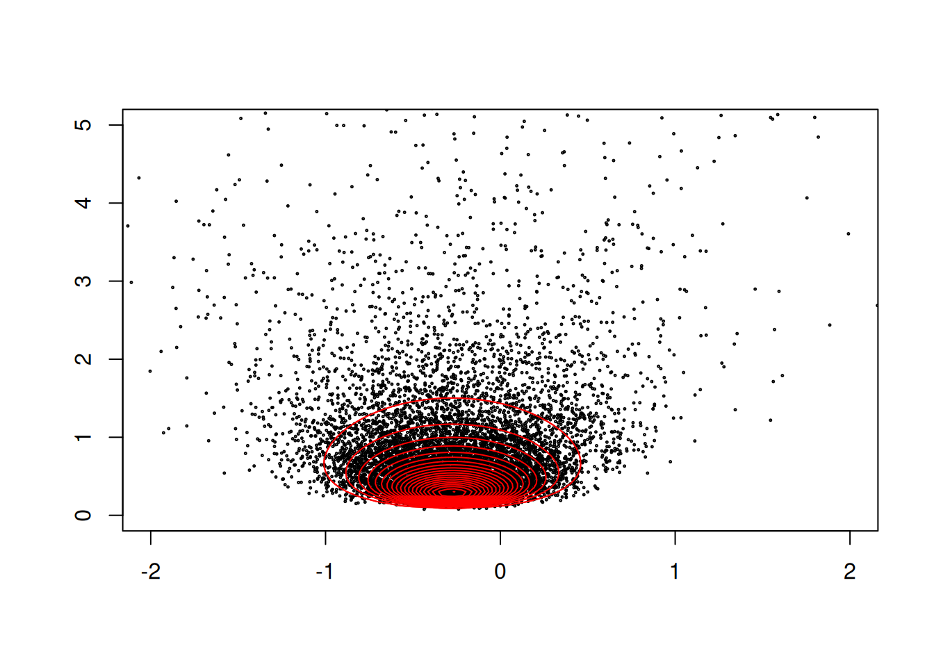
Figure 2.7: The posterior distribution \(Pr(\mu, \sigma^{2} | {\bf y})\). The black dots are samples from the posterior using MCMC, and the red contours are calculated by evaluating the posterior density on a grid of parameter values. The contours are normalised so that the posterior mode has a value of one.

and we see that MCMCglmm is sampling the same distribution as the posterior distribution calculated on a grid of possible parameter values (Figure 2.7).

A very nice property of MCMC is that we can calculate probabilities from the output without having to explicitly perform integration. Earlier we calculated the probability that the mean lay between \(\pm2\) and the variance was less than 5 (\(\texttt{p.square/C}=\) 0.982). Because MCMC has sampled the posterior distribution randomly, this probability will be equal to the expected probability that we have drawn an MCMC sample from the region. We can obtain an estimate of this by seeing what proportion of our actual samples lie in this square:

prop.table(table(m1a.2$Sol > -2 & m1a.2$Sol < 2 & m1a.2$VCV < 5))

## 
##  FALSE   TRUE 
## 0.0196 0.9804

There is Monte Carlo error in the answer (0.980) but if we collect a large number of samples then this can be minimised.

2.4.1 Marginal Posterior Distribution

The marginal distribution is often of primary interest in statistical inference, because it represents our knowledge about a parameter given the data:

\[Pr(\sigma^{2} | {\bf y}) = \int Pr(\mu, \sigma^{2} | {\bf y})d\mu \label{marg-eq} \tag{2.2}\]

after averaging over any nuisance parameters, such as the mean in this case.

Using MCMC, we can obtain the marginal distribution of the variance by simply evaluating the draws in VCV ignoring (averaging over) the draws in Sol:

hist(m1a.2$VCV)
abline(v = Best["var"], col = "red")

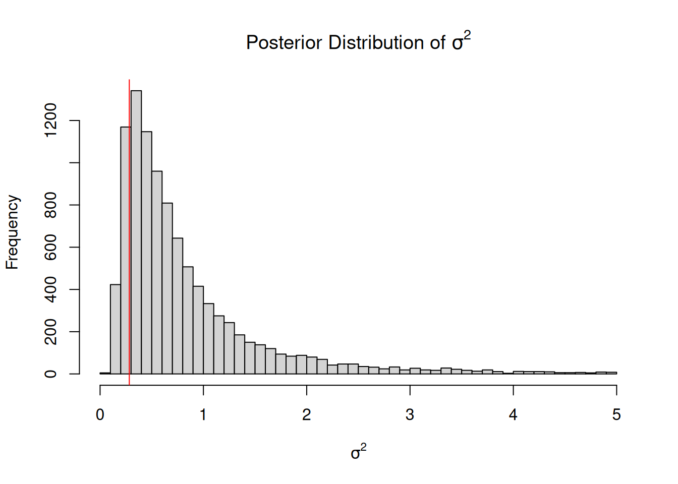
Figure 2.8: Histogram of samples from the marginal distribution of the variance \(Pr(\sigma^{2} | {\bf y})\) using MCMC. The vertical line is the joint posterior mode, which differs slightly from the marginal posterior mode (the peak of the marginal distribution).

In this example the marginal mode and the joint mode are very similar, although this is not necessarily the case and can depend on both the data and the prior. Section 2.6 covers properties of the inverse-Wishart prior in detail.

2.4.2 Credible Intervals

2.5 MCMC

In order to be confident that \(\texttt{MCMCglmm}\) has successfully sampled the posterior distribution it will be necessary to have a basic understanding of how MCMC works. The aim of MCMC is to sample parameter values from their posterior distribution, shown exactly (up to proportionality) in Figure 2.6. In all but the very simplest cases this distribution is not of a known form and we cannot sample from it directly by using functions such as rnorm. However we can set up a random walk in parameter space such that the chance a walker visits a particular set of parameter values is proportional to their posterior density. Importantly, this can done without needing to normalise the posterior density by \(C\).

2.5.1 Starting values

First we need to initialise the chain and specify a set of parameter values from which the chain can start moving through parameter space. In practice, it’s generally a good idea to start the chain in region of relatively high probability. Although starting configurations can be set by the user using the start argument, in general the heuristic techniques used by \(\texttt{MCMCglmm}\) seem to work quite well. We will denote the parameter values of the starting configuration (time \(t=0\)) as \(\mu_{t=0}\) and \({\sigma^{2}}_{t=0}\). There are several ways in which we can get the chain to move in parameter space, and the main techniques used in \(\texttt{MCMCglmm}\) are Gibbs sampling and Metropolis-Hastings updates. To illustrate, it will be easier to turn the contour plot of the posterior distribution into a perspective plot (Figure 2.9).

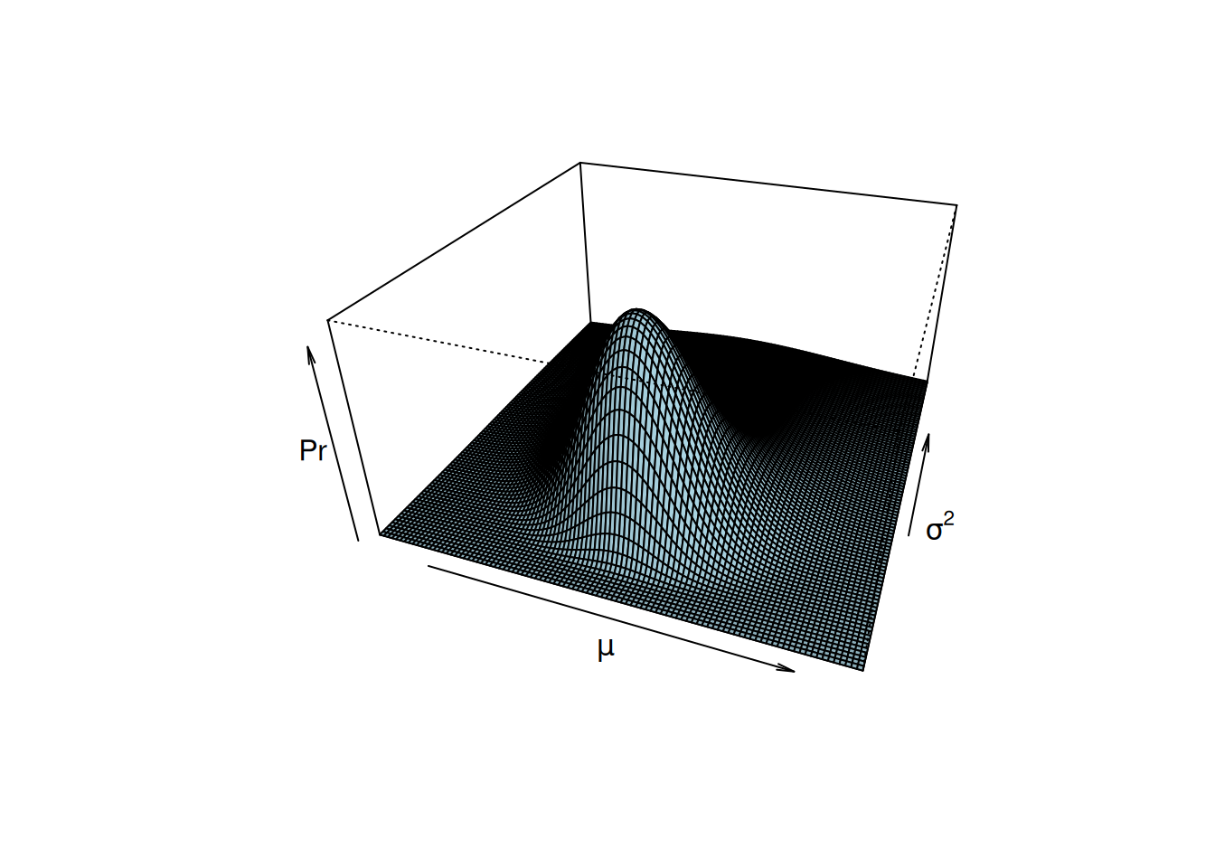
Figure 2.9: The posterior distribution \(Pr(\mu, \sigma^{2} | {\bf y})\). This perspective plot is equivalent to the contour plot in Figure 2.6 but it has been normalised by \(C\) and is equal to, not just proportional to, the posterior density.

2.5.2 Metropolis-Hastings updates

After initialising the chain we need to decide where to go next, and this decision is based on two rules. First we have to generate a candidate destination, and then we need to decide whether to go there or stay where we are. There are many ways in which we could generate candidate parameter values, and \(\texttt{MCMCglmm}\) uses a well tested and simple method. A random set of coordinates are picked from a multivariate normal distribution that is centred on the initial coordinates \(\mu_{t=0}\) and \(\sigma^{2}_{t=0}\). We will denote this new set of parameter values as \(\mu_{new}\) and \(\sigma^{2}_{new}\). The question then remains whether to move to this new set of parameter values or remain at our current parameter values now designated as old \(\mu_{old}=\mu_{t=0}\) and \(\sigma^{2}_{old}=\sigma^{2}_{t=0}\). If the posterior probability for the new set of parameter values is greater, then the chain moves to this new set of parameters and the chain has successfully completed an iteration: (\(\mu_{t=1} = \mu_{new}\) and \(\sigma^{2}_{t=1}=\sigma^{2}_{new}\)). If the new set of parameter values has a lower posterior probability then the chain may move there, but not all the time. The probability that the chain moves to low lying areas, is determined by the relative difference between the old and new posterior probabilities. If the posterior probability for \(\mu_{new}\) and \(\sigma^{2}_{new}\) is 5 times less than the posterior probability for \(\mu_{old}\) and \(\sigma^{2}_{old}\), then the chain would move to the new set of parameter values 1 in 5 times. If the move is successful then we set \(\mu_{t=1} = \mu_{new}\) and \(\sigma^{2}_{t=1}=\sigma^{2}_{new}\) as before, and if the move is unsuccessful then the chain stays where it is (\(\mu_{t=1} = \mu_{old}\) and \(\sigma^{2}_{t=1}=\sigma^{2}_{old}\)). Note that we only need to know the posterior density up to proportionality to make these calculations (i.e we could use likprior directly without knowing \(C\)). Using these rules we can record where the chain has travelled and generate an approximation of the posterior distribution. Basically, a histogram of Figure 2.9.

Why Metropolis-Hastings updates work can perhaps be more easily understood in terms of a simpler toy example. Imagine we had a strong prior such that only two sets of parameter values had positive posterior probability: Set A (\(\mu_A\) an \(\sigma^2_A\)) with a posterior probability 5 times that of Set B. If the chain is currently at Set A then the candidate parameter values will be Set B and vice-versa. Since we move from Set A to Set B 20% of the time and we move from Set B to Set A 100% of the time, the odds of being in Set A versus Set B is 1:0.2 which is exactly equal to their posterior odds of 5:1.

2.5.3 Gibbs Sampling

Gibbs sampling is a special case of Metropolis-Hastings updating, and \(\texttt{MCMCglmm}\) uses Gibbs sampling to update most parameters. In the Metropolis-Hastings example above, the Markov Chain was allowed to move in both directions of parameter space simultaneously. An equally valid approach would have been to set up two Metropolis-Hastings schemes where the chain was first allowed to move along the \(\mu\) axis, and then along the \(\sigma^{2}\) axis. In Figure 2.10 I have cut the posterior distribution of Figure 2.9 in half, and the edge of the surface facing left is the conditional distribution of \(\mu\) given that \(\sigma^{2}=1\):

\[Pr(\mu |\sigma^{2}=1, \boldsymbol{\mathbf{y}}).\]

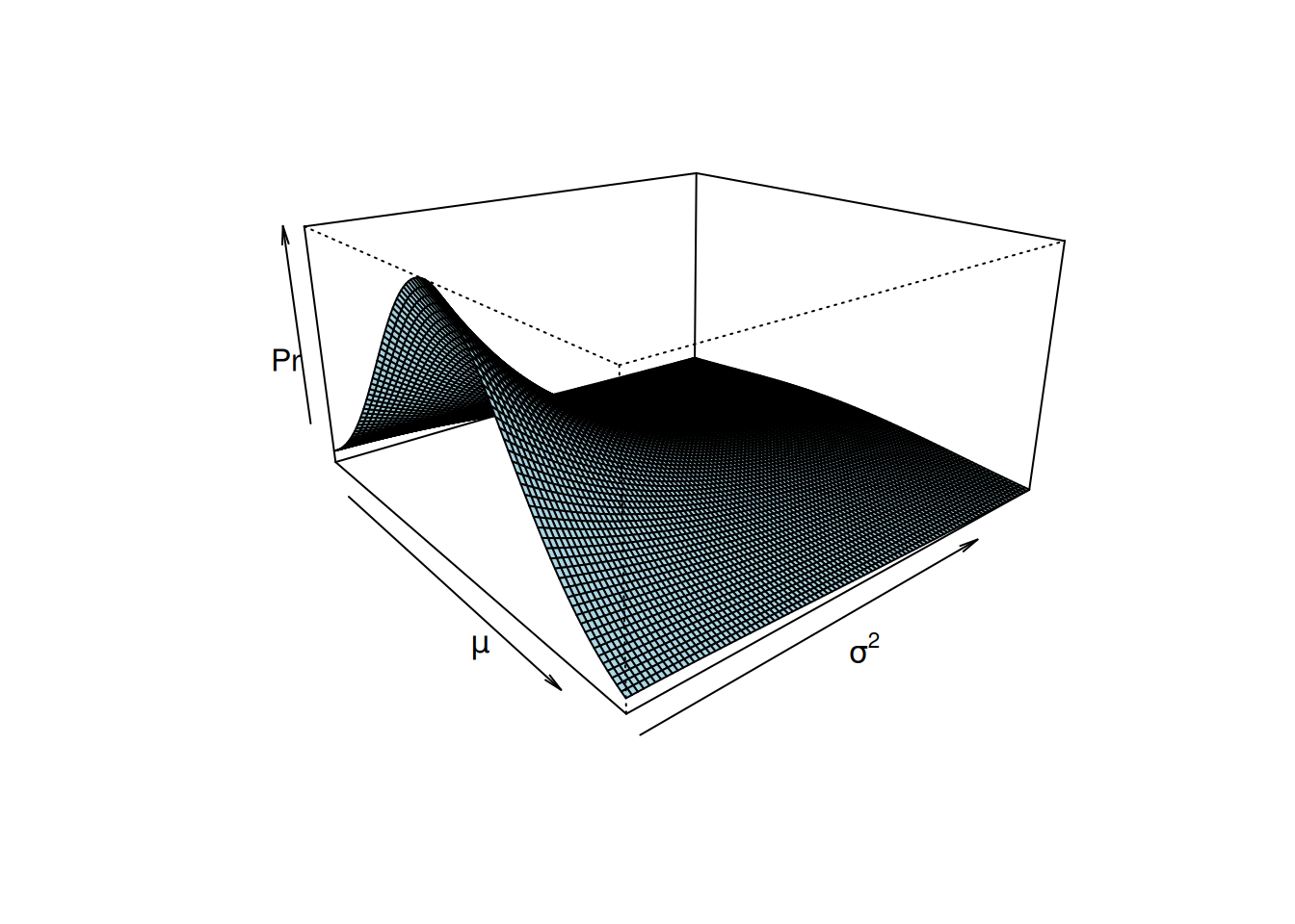
Figure 2.10: The posterior distribution \(Pr(\mu, \sigma^{2} | {\bf y})\), but only for values of \(\sigma^{2}\) between 1 and 5, rather than 0 to 5 (Figure 2.9. The edge of the surface facing left is the conditional distribution of the mean when \(\sigma^{2}=1\) (\(Pr(\mu | {\bf y}, \sigma^{2}=1)\)). This conditional distribution follows a normal distribution.

If we were using Metropolis-Hastings updates to sample \(\mu\) we would need to evaluate this density, which may be much simpler than evaluating the full density. In fact for some cases, the equation that describes this conditional distribution can be derived despite the equation for the complete joint distribution of Figure 2.9 remaining unknown. When the conditional distribution of \(\mu\) is known we can use Gibbs sampling. Lets say the chain at a particular iteration is located at \(\sigma^{2}=1\). If we updated \(\mu\) using a Metropolis-Hastings algorithm we would generate a candidate value and evaluate its relative probability compared to the old value. This procedure would take place in the slice of posterior facing left in Figure 2.10. However, because we know the actual equation for this slice we can just generate a new value of \(\mu\) directly. This is Gibbs sampling. The slice of the posterior that we can see in Figure 2.10 actually has a normal distribution. Because of the weak prior this normal distribution has a mean close to the mean of \(\bf{y}\) and a variance close to \(\frac{\sigma^{2}}{n} = \frac{1}{n}\). Gibbs sampling can be much more efficient than Metropolis-Hastings updates, especially when high dimensional conditional distributions are known, as is typical in GLMMs. A technical description of the sampling schemes used by \(\texttt{MCMCglmm}\) is given in the Chapter @ref(#technical), but is perhaps not important to know.

2.5.4 MCMC Diagnostics

When fitting a model using \(\texttt{MCMCglmm}\) the parameter values through which the Markov chain has travelled are stored and returned. The length of the chain (the number of iterations) can be specified using the nitt argument¹ (the default is 13,000), and should be long enough so that the posterior approximation is valid. If we had known the joint posterior distribution in Figure 2.9 we could have sampled directly from the posterior. If this had been the case, each successive value in the Markov chain would be independent of the previous value after conditioning on the data, \({\bf y}\), and a thousand iterations of the chain would have produced a histogram that resembled Figure 2.9 very closely. However, generally we do not know the joint posterior distribution of the parameters, and for this reason the parameter values of the Markov chain at successive iterations are usually not independent and care needs to be taken regarding the validity of the approximation. \(\texttt{MCMCglmm}\) returns the Markov chain as mcmc objects, which can be analysed using the coda package. The function autocorr from the package \(\texttt{coda}\) reports the level of non-independence between successive samples in the chain:

autocorr(m1a.2$Sol)

## , , (Intercept)
## 
##         (Intercept)
## Lag 0  1.0000000000
## Lag 1  0.0295393869
## Lag 5  0.0069888310
## Lag 10 0.0200379700
## Lag 50 0.0009886787

autocorr(m1a.2$VCV)

## , , units
## 
##                units
## Lag 0   1.0000000000
## Lag 1   0.2473917848
## Lag 5   0.0082937460
## Lag 10 -0.0132076992
## Lag 50 -0.0007171886

The correlation between successive samples is low for the mean (0.030) but a bit high for the variance (0.247). When auto-correlation is high we effectively have fewer samples from the posterior than we have saved. The function effectiveSize, also from \(\texttt{coda}\), reports the effective number of samples saved - if the autocorrelation could be made zero this would be the number of samples required to give the same precision on the posterior mean. For the variance, the effective sample size is 6248 quite a bit less than the number of stored posterior samples 10000. When the effective sample size is low the chain needs to be run for longer, and this can lead to storage problems for high dimensional problems. The argument thin can be passed to \(\texttt{MCMCglmm}\) specifying the intervals at which the Markov chain is stored. In model m1a.2 we specified thin=1 meaning we stored every iteration (the default is thin=10). I usually aim to store 1,000-2,000 effective posterior samples with the autocorrelation between successive stored samples less than 0.1.

The approximation obtained from the Markov chain is conditional on the set of parameter values that were used to initialise the chain. In many cases the first iterations show a strong dependence on the starting parametrisation, but as the chain progresses this dependence may be lost. As the dependence on the starting parametrisation diminishes the chain is said to converge and the argument burnin can be passed to MCMCped specifying the number of iterations which must pass before samples are stored. The default burn-in period is 3,000 iterations. Assessing convergence of the chain is notoriously difficult, but visual inspection and diagnostic tools such as gelman.diag often suffice. For difficult models, running several chains from different starting values and ensuring they have all converged on the same distribution is a good idea.

plot(m1a.2$Sol)

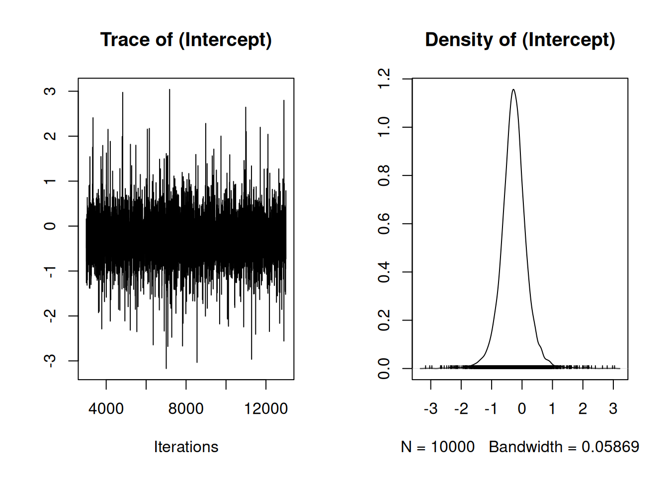
Figure 2.11: Summary plot of the Markov Chain for the intercept. The left plot is a trace of the sampled posterior, and can be thought of as a time-series. The right plot is a density estimate, and can be thought of a smoothed histogram approximating the posterior.

On the left of Figure 2.11 is a time-series of the parameter as the MCMC iterates, and on the right is a posterior density estimate of the parameter (a smoothed histogram of the output). If the model has converged there should be no trend in the time-series. The equivalent plot for the variance is a little hard to see on the original scale, but on the log scale the chain looks good (Figure 2.12:

plot(log(m1a.2$VCV))

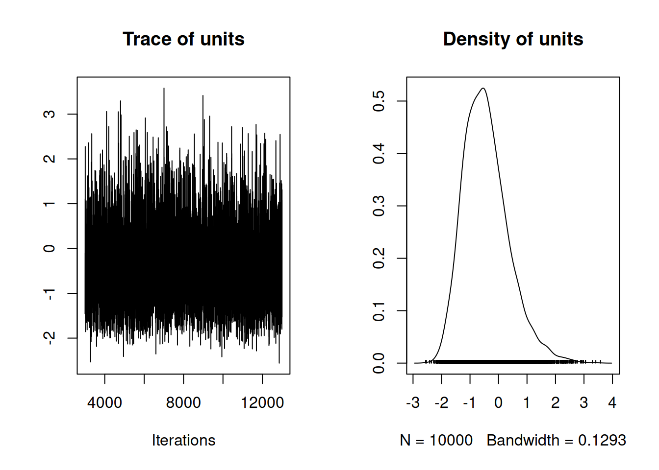
Figure 2.12: Summary plot of the Markov Chain for the logged variance. The logged variance was plotted rather than the variance because it was easier to visualise. The left plot is a trace of the sampled posterior, and can be thought of as a time-series. The right plot is a density estimate, and can be thought of a smoothed histogram approximating the posterior.

2.6 Priors for Residual Variances

\(\texttt{MCMCglmm}\) uses an inverse-Wishart prior for the residual variance and so here will cover the properties of the scalar inverse-Wishart distribution and prior. Section 5.3 can be consulted for inverse-Wishart covariance matrices. For random effect (co)variances it is possible to use scaled non-central \(F\)-distribution priors which is strongly recommended (see Section 4.6).

For a single variance, the inverse-Wishart prior is parameterised through the parameters \(\texttt{V}\) and \(\texttt{nu}\) in MCMCglmm. The MCMCglmm parameterisation of the inverse-Wishart is not standard but I find it intuitive: the prior information is equivalent to observing \(\texttt{nu}\) residuals with variance \(\texttt{V}\). Consequently, the distribution concentrates on \(\texttt{V}\) as the degree of belief parameter, \(\texttt{nu}\) increases. The distribution tends to be right skewed when \(\texttt{nu}\) is not very large, with a mode of \(\texttt{V}\frac{\texttt{nu}}{\texttt{nu}+2}\) but a mean of \(\texttt{V}\frac{\texttt{nu}}{\texttt{nu}-2}\) (which is not defined for \(\texttt{nu}<2\)). Figure 2.13 plots the probability density functions holding \(\texttt{V}\) equal to one but with \(\texttt{nu}\) varying.

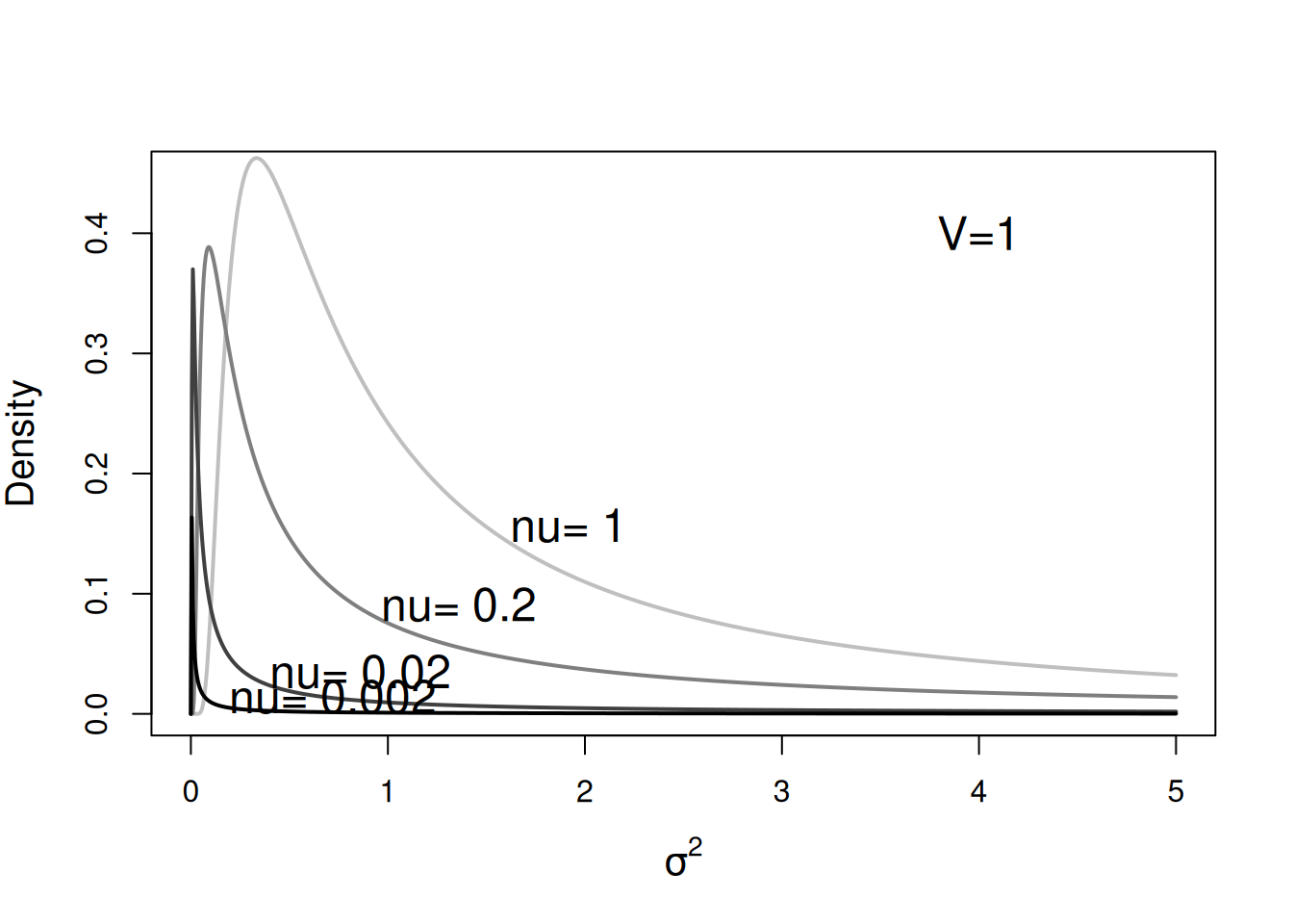
Figure 2.13: Probability density function for a univariate inverse-Wishart with the variance at the limit set to 1 (\(\texttt{V}=1\)) and varying degree of belief parameter (\(\texttt{nu}\)). With \(\texttt{V}=1\) these distributions are equivalent to inverse gamma distributions with shape and scale parameters set to \(\texttt{nu}\)/2.

For single variances the inverse-gamma is a special case of the inverse-Wishart², and with \(\texttt{V}=1\), the shape and scale of the inverse-gamma are both equal to \(\texttt{nu}/2\). The inverse-gamma with shape and scale equal to 0.001 used to be commonly used. The motivation behind the prior was that making \(\texttt{nu}\) small would result in a less influential prior because is was equivalent to only observing 0.2% (\(\texttt{nu}=0.002\)) of a residual a priori. Setting \(\texttt{nu}=0\) was avoided because this does not define a valid distribution. A probability distribution must integrate to one because a variable must have some value, and this condition is not met when setting \(\texttt{nu}=0\). The prior distribution is said to be improper. In the example here, where \(\texttt{V}\) is a single variance, the prior is only proper when \(\texttt{V}>0\) and \(\texttt{nu}>0\). Although improper priors do not specify valid prior distributions and therefore the Bayesian credentials of any model may be questionable, \(\texttt{MCMCglmm}\) does allow them as they have some useful properties.

2.6.1 Improper Priors

When improper priors are used their are two potential problems that may be encountered. The first is that if the data do not contain enough information, the posterior distribution itself may be improper, and any results obtained from \(\texttt{MCMCglmm}\) will be meaningless. In addition, with proper priors there is a zero probability of a variance component being exactly zero but this is not necessarily the case with improper priors. This can produce numerical problems (trying to divide through by zero) and can also result in a reducible chain. A reducible chain is one which gets ‘stuck’ at some parameter value(s) and cannot escape. This is usually obvious from the mcmc plots but \(\texttt{MCMCglmm}\) will often terminate before the analysis has finished with an error message of the form:

ill-conditioned G/R structure: use proper priors ...

However, improper priors do have some useful properties and in fact the default prior for the variances in has \(\texttt{nu}=0\) (the value of \(\texttt{V}\) is irrelevant). It is tempting to think that this prior is flat for the variance³, but it is in fact flat for the log-variance and therefore puts more weight on small values than a prior that is flat on the variance (Figure 2.14) - see Section 2.7.

prior.m1a.3 <- list(R = list(V = 1, nu = 0))
m1a.3 <- MCMCglmm(y ~ 1, data = Ndata, thin = 1, prior = prior.m1a.3)

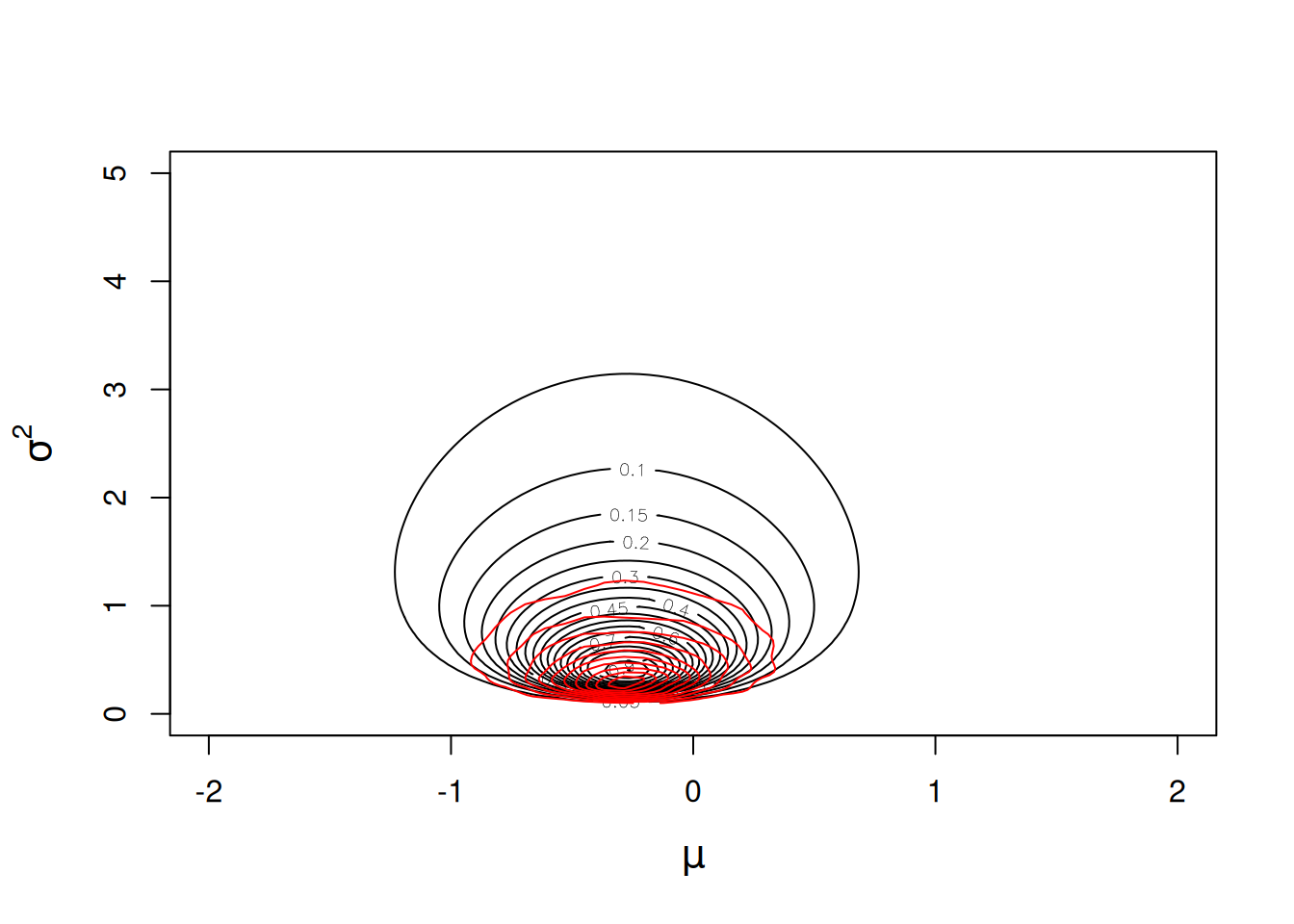
Figure 2.14: Likelihood surface for the likelihood \(Pr({\bf y}|\mu, \sigma^{2})\) in black, and an MCMC approximation for the posterior distribution \(Pr(\mu, \sigma^{2} | {\bf y})\) in red. The likelihood has been normalised so that the maximum likelihood has a value of one, and the posterior distribution has been normalised so that the posterior mode has a value of one. An almost flat prior was used for the mean \(Pr(\mu)\sim N(0, 10^8)\) and a flat prior was used for the log-variance \(Pr(\sigma^{2})\sim IW(\texttt{V}=1, \texttt{nu}=0)\)).

Consequently, the mode of the marginal posterior distribution lies even below the ML estimate 2.15.

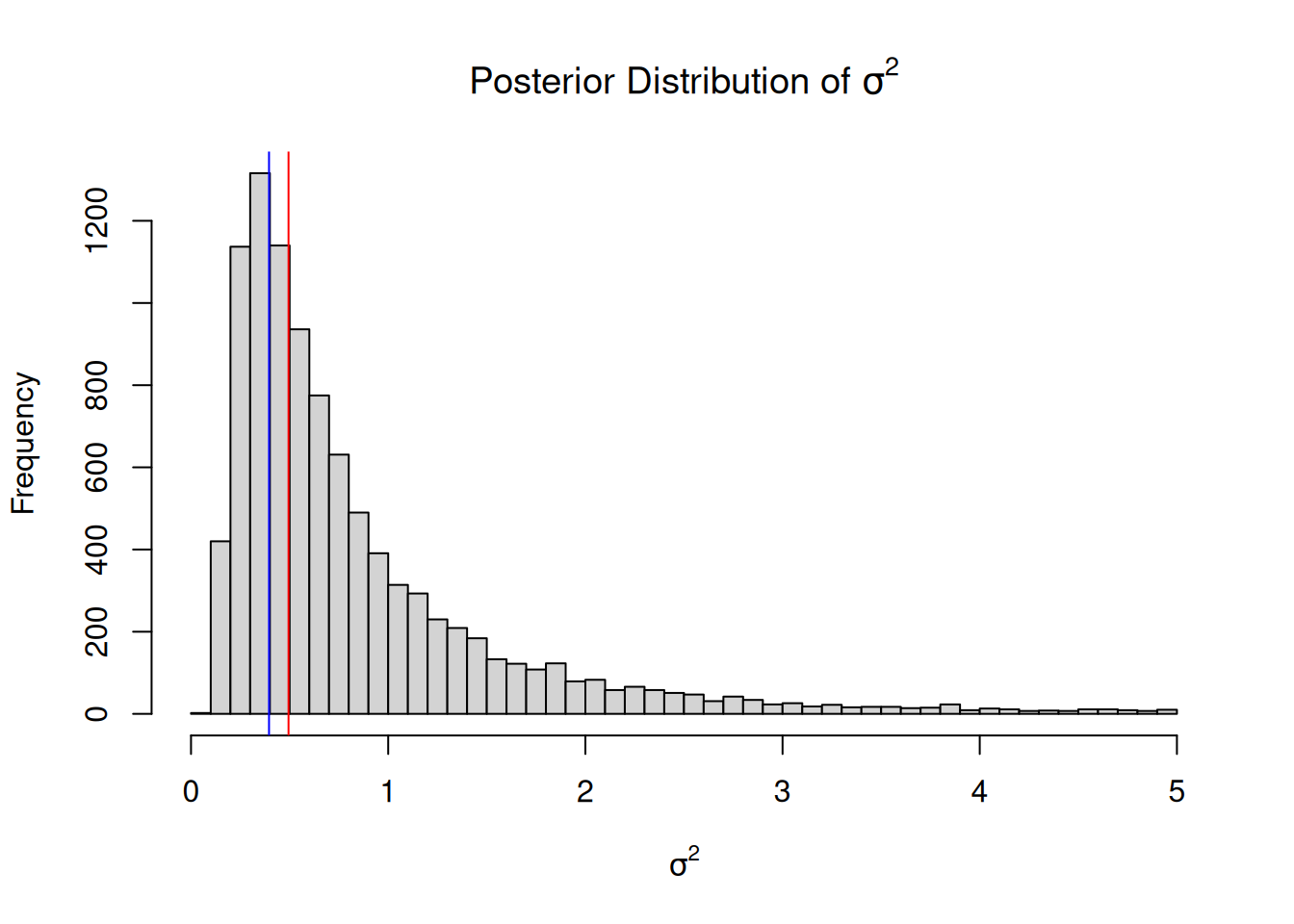
Figure 2.15: An MCMC approximation for the marginal posterior distribution of the variance \(Pr(\sigma^{2} | {\bf y})\). A non-informative prior specification was used (\(Pr(\mu)\sim N(0, 10^8)\) and \(Pr(\sigma^{2})\sim IW(\texttt{V}=0, \texttt{nu}=0)\)). The ML and REML estimates are plotted in blue and red,m respectively.

Although inverse-Wishart distributions with negative degree of belief parameters are not defined, the resulting posterior distribution can be defined and proper if there is sufficient replication. When \(\texttt{V}=0\) and \(\texttt{nu}=-1\) we have a flat prior on the standard deviation over the interval \((0,\infty]\). When \(\texttt{V}=0\) and \(\texttt{nu}=-2\) we have a flat prior on the variance. Since the default prior for the mean is normal with a very large variance (\(10^8\)) the prior for the mean is also essentially flat, resulting in a prior probability that is proportional to some constant for all possible parameter values. The posterior density in such cases is equal to the likelihood:

\[Pr(\mu, \sigma^{2} | {\bf y}) \propto Pr({\bf y} | \mu, \sigma^{2}) \label{fprior-eq} \tag{2.3}\]

We can overlay the joint posterior distribution on the likelihood surface (Figure 2.16) and see that the two things are in close agreement, up to Monte Carlo error.

prior.m1a.4 <- list(R = list(V = 1e-16, nu = -2))
m1a.4 <- MCMCglmm(y ~ 1, data = Ndata, thin = 1, prior = prior.m1a.4)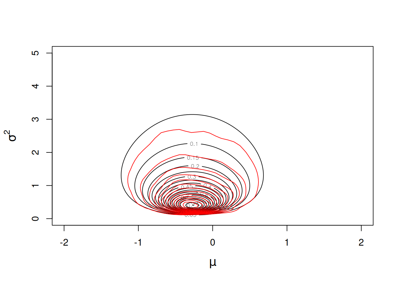

Figure 2.16: Likelihood surface for the likelihood \(Pr({\bf y}|\mu, \sigma^{2})\) in black, and an MCMC approximation for the posterior distribution \(Pr(\mu, \sigma^{2} | {\bf y})\) in red. The likelihood has been normalised so that the maximum likelihood has a value of one, and the posterior distribution has been normalised so that the posterior mode has a value of one. Almost flat priors were used for the mean (\(Pr(\mu)\sim N(0, 10^8)\) and the variance \(Pr(\sigma^{2})\sim IW(\texttt{V}=10^{-16}, \texttt{nu}=-2)\)) and so the posterior distribution is equivalent to the likelihood.

Here, the joint posterior mode coincides with the ML estimates, as expected (Figure 2.16). In addition, the mode of the marginal distribution for the variance is equivalent to the REML estimator (See Figure 2.17). Indeed, the REML estimator can be seen as marginalising the mean under a flat prior, and for this reason is sometimes referred to as the marginal likelihood rather than the restricted likelihood (REML).

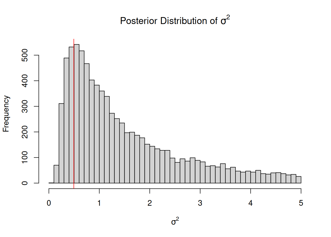
Figure 2.17: An MCMC approximation for the marginal posterior distribution of the variance \(Pr(\sigma^{2} | {\bf y})\). An almost flat prior specification was used (\(Pr(\mu)\sim N(0, 10^8)\) and \(Pr(\sigma^{2})\sim IW(\texttt{V}=10^{-16}, \texttt{nu}=-2)\)) and the REML estimator of the variance (red line) coincides with the marginal posterior mode.

2.7 Transformations

Sometimes we would like to know the posterior distribution for some transformation of the parameters. For example, we may wish to obtain the posterior distribution for \(\log(\sigma^2)\). With MCMC this is easy - we can just transform the posterior samples (i.e. log(m1a.2$VCV)) and treat these as we would any other set of posterior samples. However, it is useful to understand how probabilities are expected to behave under these transformations. The key idea is that the probability of some function of \(x\), \(f(x)\), is equal to the probability of \(x\) divided by the Jacobian. When the transform only involves single parameters the Jacobian is \(|df(x)/dx|\) which for the log-transform is \(1/x\). For model m1a.3 we used an inverse-Wishart prior with \(\texttt{V=1}\) and \(\texttt{nu=0}\). The posterior density is plotted in Figure 2.14 and does not appear to coincide with the likelihood - there is more posterior density at small values of \(\sigma^2\)

However, this is because the posterior density is expressed for \(\sigma^2\) and the prior is only flat in \(log(\sigma^2)\). By multiplying the posterior density for \(\sigma^2\) by \(\sigma^2\) (i.e. dividing by \(1/x\) where \(x\) is \(\sigma^2\)) we would obtain the joint density of \(\mu\) and \(log(\sigma^2)\). This would reduce the density for small values of \(\sigma^2\) and increase the density for large values (since the density is scaled by \(\sigma^2\)). Indeed, plotting the posterior distribution of \(log(\sigma^2)\) shows this effect and the posterior is in agreement with the likelihood, as expected (Figure 2.18).

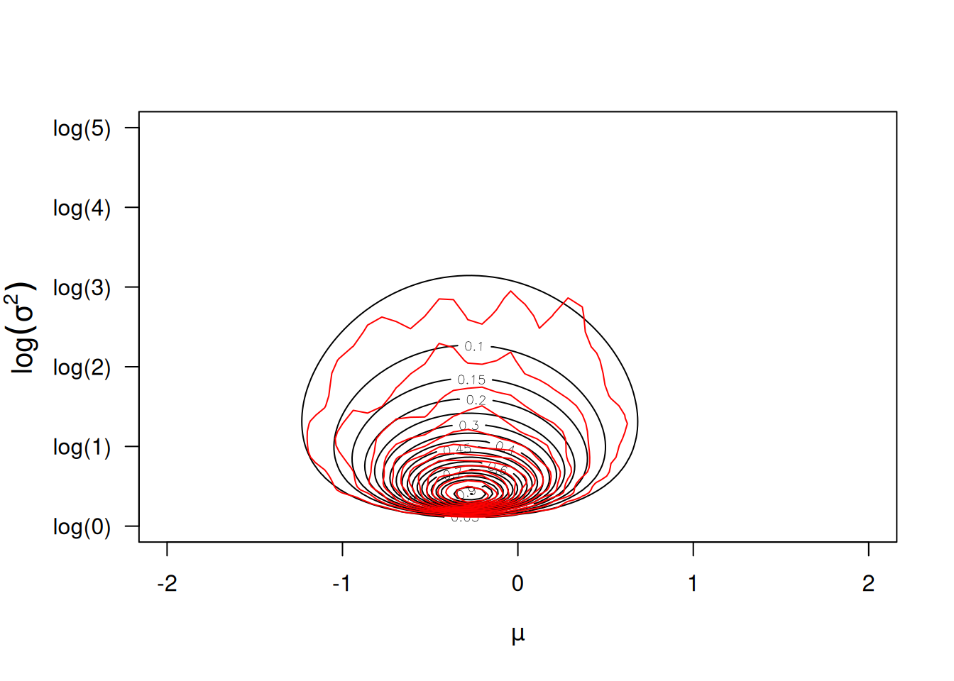
Figure 2.18: Likelihood surface for the likelihood \(Pr({\bf y}|\mu, \log(\sigma^{2}))\) in black, and an MCMC approximation for the posterior distribution \(Pr(\mu, \log(\sigma^{2}) | {\bf y})\) in red. An almost flat prior was used for the mean \(Pr(\mu)\sim N(0, 10^8)\) and a flat prior was used for the log-variance \(Pr(\sigma^{2})\sim IW(\texttt{V}=1, \texttt{nu}=0)\).

---

1. The double t is because I cannot spell.↩︎

2. The inverse gamma is a special case of the inverse-Wishart, although it is parametrised using \(\texttt{shape}\) and \(\texttt{scale}\), where \(\texttt{nu}=2\ast\texttt{shape}\) and \(\texttt{V} = \frac{\texttt{scale}}{\texttt{shape}}\) (or \(\texttt{shape} = \frac{\texttt{nu}}{2}\) and \(\texttt{scale} = \texttt{V}\frac{\texttt{nu}}{2}\)). There is no density function for the inverse-gamma in base R. However, the prior specification can be passed to the function \(\texttt{dprior}\) to obtain the density: for example, dprior(1, prior=list(V=1, nu=0.002)).↩︎

3. Embarrassingly, I claimed that \(\texttt{V=1}\) and \(\texttt{nu=0}\) was flat in the original CourseNotes and I had forgotten to rescale the posterior density by the Jacobian when generating the equivalent contour plot to Figure 2.14 (which is computed on values of \(\textrm{log}(\sigma^2)\) for better results, and then transformed).↩︎