7 Multi-response Models
So far we have only fitted models to a single response variable, and even then, each response variable came from a distribution that only required one location parameter to be estimated, such as the mean of the Poisson or the probability of the binomial. In this section we will first cover multi-response models and then move on to models of multi-parameter distributions.
Since they are much less widely used than single-response models, let’s start by motivating why anyone would want to use them. Imagine we knew how much money 200 people had spent on their holiday and on their car in each of four years, and we want to know whether a relationship exists between the two. A simple correlation would be one possibility, but then how do we control for the repeated measures? An often used solution to this problem is to choose one variable as the response (lets say the amount spent on a car) and have the other variable as a predictor (the amount spent on a holiday) for which a fixed effect is estimated. The choice is essentially arbitrary, highlighting the belief that any relationship between the two types of spending maybe in part due to unmeasured variables, rather than being completely causal.
In practice does this matter? Let’s imagine there was only one unmeasured variable: disposable income. There are repeatable differences between individuals in their disposable income, but also some variation within individuals across the four years. Likewise, people vary in what proportion of their disposable income they are willing to spend on a holiday versus a car, but this also changes from year to year. We can simulate some toy data to get a feel for the issues:
id<-gl(200,4)   # 200 people recorded four times

av_wealth<-rlnorm(200, 0, 1)
ac_wealth<-rlnorm(800, log(av_wealth[id]), 1/4)
# expected disposable incomes + some year to year variation

av_ratio<-rbeta(200,10,10)
ac_ratio<-rbeta(800, 3*(av_ratio[id]), 3*(1-av_ratio[id]))
# expected proportion spent on car + some year to year variation

y.car<-ac_wealth*ac_ratio      # disposable income * proportion spent on car
y.hol<-ac_wealth*(1-ac_ratio)  # disposable income * proportion spent on holiday

Spending<-data.frame(y.hol=log(y.hol), y.car=log(y.car), id=id)
A simple model suggests the two types of spending (on the log-scale) are positively related:
##
##  Iterations = 3001:12991
##  Thinning interval  = 10
##  Sample size  = 1000
##
##  DIC: 2715.422
##
##  R-structure:  ~units
##
##       post.mean l-95% CI u-95% CI eff.samp
## units     1.738    1.581    1.902     1000
##
##  Location effects: y.car ~ y.hol
##
##             post.mean l-95% CI u-95% CI eff.samp  pMCMC
## (Intercept)   -0.7092  -0.8365  -0.6039     1000 <0.001 ***
## y.hol          0.2807   0.2137   0.3474     1000 <0.001 ***
## ---
## Signif. codes:  0 '***' 0.001 '**' 0.01 '*' 0.05 '.' 0.1 ' ' 1
This conclusion seems to be supported by just looking at a scatter plot of the two variables (Figure 7.1).
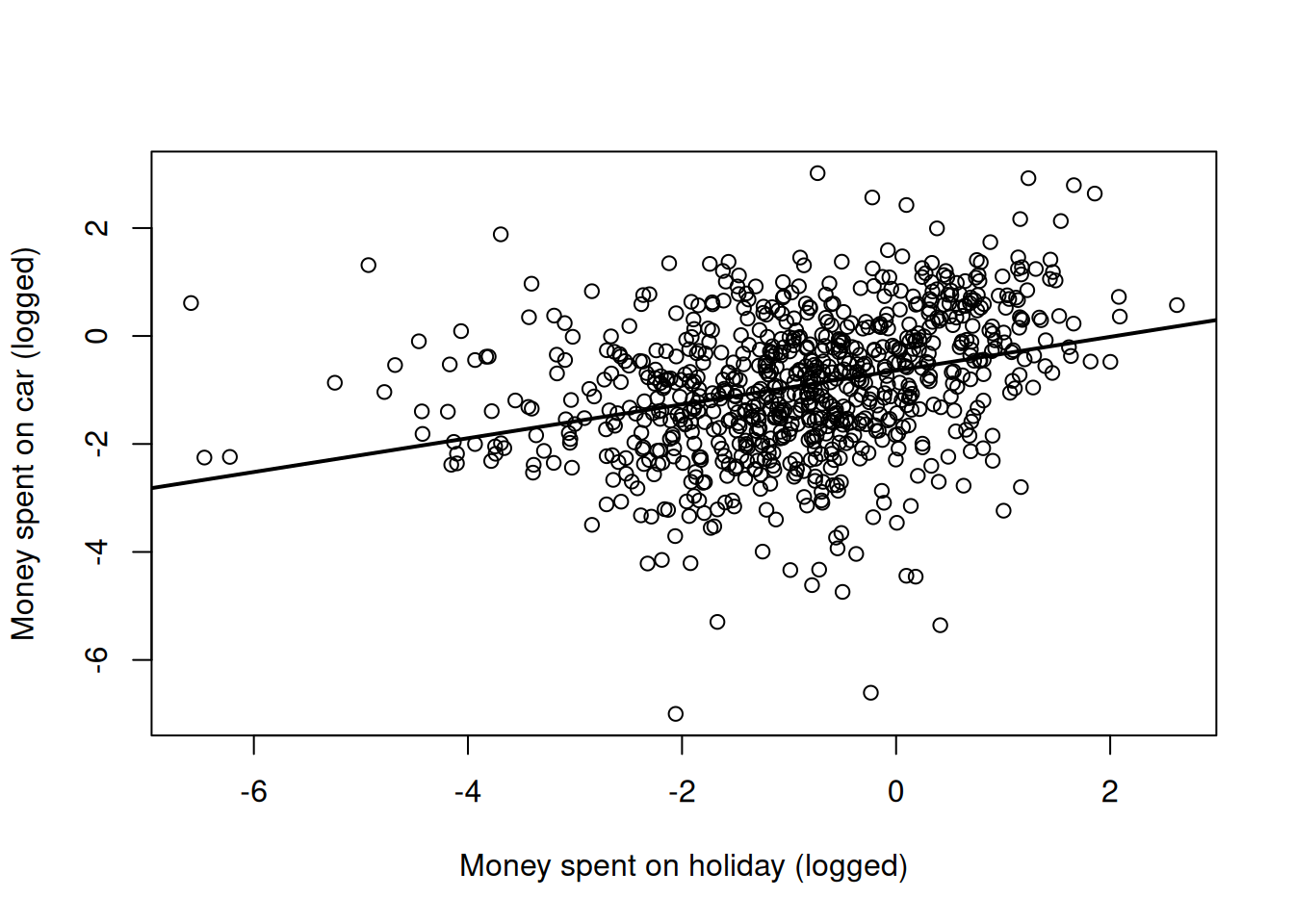
Figure 7.1: Money spent on car versus money spent on holiday (both logged) with the regression line from a simple regression (model mspending.1)
An obvious problem with the model is that we have repeated measures (the spending habits of each individual have been recorded for each of four years) and yet we haven’t dealt with any possible non-independence. We can remedy this by fitting id effects as random:
##
##  Iterations = 3001:12991
##  Thinning interval  = 10
##  Sample size  = 1000
##
##  DIC: 2039.254
##
##  G-structure:  ~id
##
##    post.mean l-95% CI u-95% CI eff.samp
## id     1.792    1.339    2.176     1000
##
##  R-structure:  ~units
##
##       post.mean l-95% CI u-95% CI eff.samp
## units    0.5948    0.533   0.6699     1000
##
##  Location effects: y.car ~ y.hol
##
##             post.mean l-95% CI u-95% CI eff.samp  pMCMC
## (Intercept)   -1.2760  -1.4988  -1.0957     1000 <0.001 ***
## y.hol         -0.2992  -0.3660  -0.2240     1000 <0.001 ***
## ---
## Signif. codes:  0 '***' 0.001 '**' 0.01 '*' 0.05 '.' 0.1 ' ' 1
Strangely, and in contradiction to the scatter plot, the model suggests that spending more on a holiday means less is spent on a car - the regression slope is negative. If I hadn’t looked at the raw data, I would probably report the negative relationship and move on. But I have looked at the raw data and simply reporting a negative relationship without caveats makes me feel uneasy.
Lets proceed with a multi-response model of the problem to see what is going on. The two responses are passed as a matrix using cbind(), and the rows of this matrix are indexed by the reserved variable units, and the columns by the reserved variable trait. It is useful to think of a new data frame where the response variables have been stacked column-wise and the other predictors duplicated accordingly. Below is the original data frame on the left (Spending) and the stacked data frame on the right when cbind(y.hol, y.car) is passed as the response:
\[\begin{array}{cc} \begin{array}{cccc} &{\color{blue}{\texttt{y.hol}}}&{\color{blue}{\texttt{y.car}}}&\texttt{id}\\ {\color{red}{\texttt{1}}}&\texttt{0.888491}&\texttt{-3.320300}&\texttt{1}\\ {\color{red}{\texttt{2}}}&\texttt{-0.067398}&\texttt{0.423423}&\texttt{1}\\ \vdots&\vdots&\vdots\\ {\color{red}{\texttt{800}}}&\texttt{-1.367001}&\texttt{-2.366404}&\texttt{200}\\ \end{array}& \Longrightarrow \begin{array}{ccccc} &\texttt{y}&{\color{blue}{\texttt{trait}}}&\texttt{id}&{\color{red}{\texttt{units}}}\\ 1&\texttt{0.888491}&{\color{blue}{\texttt{y.hol}}}&\texttt{1}&{\color{red}{\texttt{1}}}\\ 2&\texttt{-0.067398}&{\color{blue}{\texttt{y.hol}}}&\texttt{1}&{\color{red}{\texttt{2}}}\\ \vdots&\vdots&\vdots&\vdots\\ 800&\texttt{-1.367001}&{\color{blue}{\texttt{y.hol}}}&\texttt{200}&{\color{red}{\texttt{800}}}\\ 801&\texttt{-3.320300}&{\color{blue}{\texttt{y.car}}}&\texttt{1}&{\color{red}{\texttt{1}}}\\ 802&\texttt{0.423423}&{\color{blue}{\texttt{y.car}}}&\texttt{1}&{\color{red}{\texttt{2}}}\\ \vdots&\vdots&\vdots&\vdots\\ 1600&\texttt{-2.366404}&{\color{blue}{\texttt{y.car}}}&\texttt{200}&{\color{red}{\texttt{800}}}\\ \end{array} \end{array} \label{multi-eq} \tag{7.1}\]
From this we can see that fitting a multi-response model is a direct extension to how we fitted models with categorical random interactions (Chapter 5):
prior.mspending.3<-list(R=IW(1, 0.002),G=F(2,1000))

mspending.3<-MCMCglmm(cbind(y.hol, y.car)~trait-1, random=~us(trait):id, rcov=~us(trait):units, data=Spending, prior=prior.mspending.3, family=c("gaussian", "gaussian"))
The only real difference is that we must now specify the distribution for each response in \(\texttt{family}\). While the interpretation of the model is identical to that covered in Chapter 5, it does take a little time to get used to working with the new categorical factor, \(\texttt{trait}\).
I have fitted a fixed \(\texttt{trait}\) effect so that the two types of spending can have different intercepts. I usually suppress the global intercept (-1) for these types of models so the second coefficient is not the difference between the intercept for the first level of \(\texttt{trait}\) (y.hol) and the second level (y.car) but the actual trait specific intercepts. Note that the levels of \(\texttt{trait}\) are ordered as they appear in the response (\(\texttt{y.hol}\) then \(\texttt{y.car}\) in this instance). A \(2\times2\) covariance matrix is estimated for the random term where the diagonal elements are the variance in consistent individual (\(\texttt{id}\)) effects for each type of spending. The off-diagonal is the covariance between these effects which if positive suggests that people that consistently spend more on their holidays consistently spend more on their cars. A \(2\times2\) residual covariance matrix is also fitted. In Section5.1.1 we fitted heterogeneous error models using idh():units which made sense for single-response models because each level of unit was specific to a particular observation and so any covariances could not be estimated. In multi-response models this is not the case because both traits have often been measured on the same observational unit and so the covariance can be measured. In the context of this example a positive covariance would indicate that in those years an individual spent a lot on their car they also spent a lot on their holiday. Let’s take a look at the model summary:
##
##  Iterations = 3001:12991
##  Thinning interval  = 10
##  Sample size  = 1000
##
##  DIC: 4218.162
##
##  G-structure:  ~us(trait):id
##
##                          post.mean l-95% CI u-95% CI eff.samp
## traity.hol:traity.hol.id     1.089   0.8438    1.358     1000
## traity.car:traity.hol.id     0.889   0.6952    1.120     1000
## traity.hol:traity.car.id     0.889   0.6952    1.120     1000
## traity.car:traity.car.id     1.158   0.9288    1.436      739
##
##  R-structure:  ~us(trait):units
##
##                             post.mean l-95% CI u-95% CI eff.samp
## traity.hol:traity.hol.units    0.8171   0.7302   0.8994     1000
## traity.car:traity.hol.units   -0.3657  -0.4360  -0.3050     1000
## traity.hol:traity.car.units   -0.3657  -0.4360  -0.3050     1000
## traity.car:traity.car.units    0.7378   0.6509   0.8166     1000
##
##  Location effects: cbind(y.hol, y.car) ~ trait - 1
##
##            post.mean l-95% CI u-95% CI eff.samp  pMCMC
## traity.hol   -0.9677  -1.1318  -0.7964     1000 <0.001 ***
## traity.car   -0.9805  -1.1497  -0.8312     1000 <0.001 ***
## ---
## Signif. codes:  0 '***' 0.001 '**' 0.01 '*' 0.05 '.' 0.1 ' ' 1
we can see that the between-individual covariance (\(\texttt{traity.car:traity.hol.id}\)) is strongly positive but the with-individual covariance (\(\texttt{traity.car:traity.hol.unit}\)) is strongly negative.
With a single predictors, a regression is defined as the covariance between the response and the predictor divided by the variance in the predictor29. We can therefore obtain the coefficients of a regression of \(\texttt{y.car}\) on \(\texttt{y.hol}\) at the level of both \(\texttt{id}\) and \(\texttt{units}\)30:
id.regression<-mspending.3$VCV[,"traity.car:traity.hol.id"]
# covariance between individuals
id.regression<-id.regression/mspending.3$VCV[, "traity.hol:traity.hol.id"]
# regression across individual

units.regression<-mspending.3$VCV[,"traity.car:traity.hol.units"]
# covariance within individuals
units.regression<-units.regression/mspending.3$VCV[,"traity.hol:traity.hol.units"]
# regression within individuals
Conceptually, the regression at the level of \(\texttt{id}\) is a regression of average expenditures across people, whereas the regression at the level of \(\texttt{units}\) is a regression of yearly expenditures within individuals. We can compare these two regression with those that we got from the single response models that did (mspending.2) or did not (mspending.1) fit \(\texttt{id}\) effects (Figure 7.2).
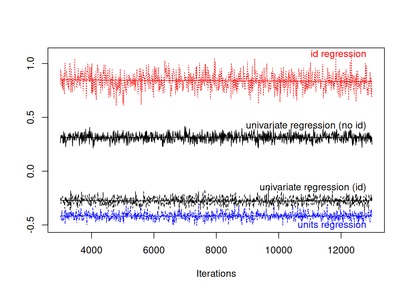
Figure 7.2: MCMC summary plot of the coefficient from a regression of car spending on holiday spending in black. The red and green traces are from a model where the regression coefficient is estimated at two levels: within an individual (blue) and across individuals (red). The relationship between the two types of spending is in part mediating by a third unmeasured variable, disposable income.
The regression coefficients differ substantially at the within individual (blue) and between individual (red) levels, and neither is entirely consistent with the regression coefficient from the single response models (black). The process by which we generated the data gives rise to this phenomenon - large variation between individuals in their disposable income means that people who are able to spend a lot on their holiday can also afford to spend a lot on their holidays (hence positive covariation between \(\texttt{id}\) effects). However, a person that spent a large proportion of their disposable income in a particular year on a holiday, must have less to spend that year on a car (hence negative residual (within year) covariation).
When fitting the simpler single-response models we make the assumption that the effect of spending money on a holiday directly effects how much you spend on a car. If this relationship was purely causal then the regression coefficients at the level of \(\texttt{id}\) and \(\texttt{units}\) would have the same expectation, and the simpler model would be justified. For example, we could simulate data where the expected car expenditure depends directly on holiday expenditure (using a regression coefficient of -0.3) with some variation around this due to between and within-individual effects:
We can fit the univariate and multivariate models to these data, and compare the regression coefficients as we did before. Figure 7.3 shows that the regression coefficients are all similar and a value of -0.3 has a reasonably high posterior probability.
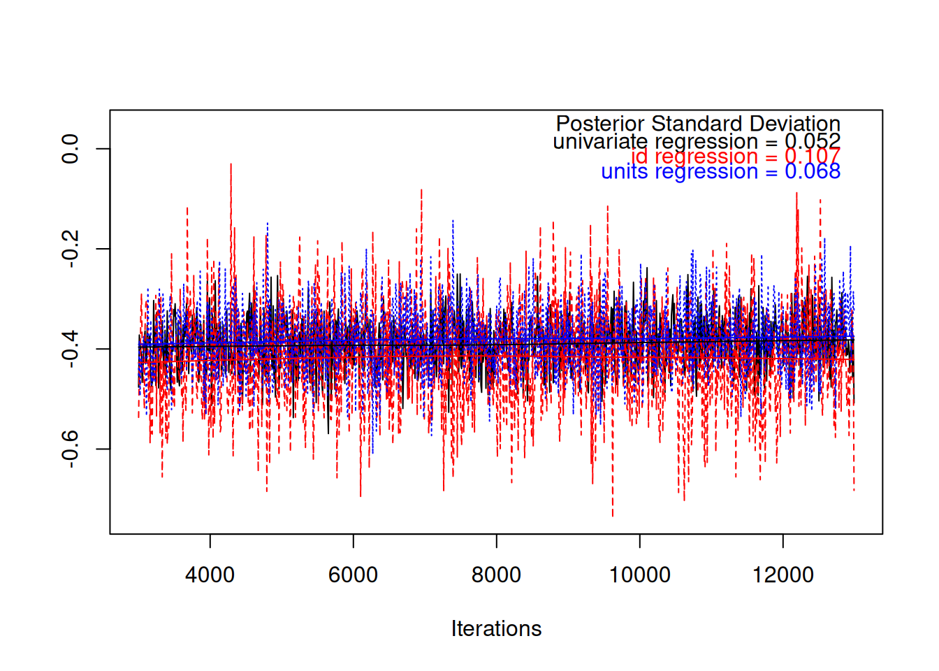
Figure 7.3: MCMC trace plot of the coefficient from a regression of car spending on holiday spending in black. The red and blue traces are from a model where the regression coefficient is estimated at two levels: within an individual (blue) and across individuals (red). In simulated data the relationship between the two types of spending is causal and the regression coefficients have the same expectation. However, the posterior standard deviation from the simple regression is smaller because information from the two different levels is pooled.
However, it should be noted that the posterior standard deviation is smaller in the simpler model because the more strict assumptions have allowed us to pool information across the two levels to get a more precise answer. This is one of the downsides of multi-response models - if the regressions at each level are the same we can get a more precise estimate using a standard single-response model. The other major benefit of the single-response model is that we only have to worry whether the conditional distribution of the response variable is modelled well (\(\texttt{y.car}\) in this case) . In a multi-response model, we have to consider whether the model for the joint distribution of all responses is doing a good job.
7.1 Multi-response Non-Gaussian Models
Model specification for multi-response models does not depend on whether the response variables are Gaussian or not. However, there is an important difference between models involving non-Gaussian variables and those involving only Gaussian variables. For Gaussian responses, the linear predictor is defined as
\[\boldsymbol{\eta} = E[{\bf y}|{\bf X}\boldsymbol{\beta}+{\bf Z}{\bf u}]\]
and any observation-level deviations from this expectation appear as \(\texttt{units}\) effects:
\[{\bf e} = {\bf y}-\boldsymbol{\eta}\]
For non-Gaussian data the linear predictor is defined
\[\boldsymbol{\eta} = E[{\bf l}|{\bf X}\boldsymbol{\beta}+{\bf Z}{\bf u}+{\bf e}]\]
where \({\bf l}\) is a vector of latent variables (Section 3.4.2). Here the \(\texttt{units}\) effects appear inside the linear predictor and model any overdispersion with respect to the named distribution. The ‘residual’ due to the named distribution is then
\[{\bf y} -\textrm{link}^{-1}(\boldsymbol{\eta})\]
Consequently, with non-Gaussian data the covariances are set up in terms of the underlying parameters of the distribution (on the link scale) not in terms of the response directly. This is not always appropriate. Let’s take the example of the Sweedish road accident data analysed in Chapter 3. We saw that the number of accidents per day can be modelled using an overdispersed Poisson. Let’s say we also had data on how much money car insurance companies paid out each day. A sensible way of modelling insurance pay-outs would to treat it as Gaussian and include the number of accidents as a covariate. However, if we analysed the accident and insurance pay-out data in a multi-response model, we would be measuring the covariance between insurance pay-outs and the expected number of accidents per day (\(l\)). Insurance companies don’t pay settlements to hypothetical accidents but actual accidents (\(\texttt{y}\)) and so the multi-response model is questionable. In contrast, let’s say we also had data on how icy the road was on each day. Here, I would be quite happy to say that iciness determines the expected number of accidents per day (\(l\)) but the actual number of accidents (\(\texttt{y}\)) will vary around this expectation. However, even here care still needs to be taken.
In Section 3.4 we saw that overdispersion arises if there are unmeasured variables that affect the response of interest. If iciness (\(\texttt{ice}\)) was an important predictor of the number of accidents, then including it as a covariate in a single-response model of the number of accidents would bring the overdsipsersion, and hence \(\sigma^2_\texttt{units}\), down. In a multi-response model we can obtain the shift in the \(\texttt{units}\) variance had we done this. The \(\texttt{units}\) variance for road accidents (\(\sigma^2_\texttt{traity.unit}\)) would be equivalent to the units variance in a single-response model without iciness as a covariate. However, \(\sigma^2_\texttt{traity.unit}-\sigma^2_\texttt{traity:traitice.unit}/\sigma^2_\texttt{traitice.unit}\) is equivalent to the units variance in the single-response model had iciness been fitted31. Let’s call this \(\sigma^2_\texttt{traity|ice.unit}\) since it is the \(\texttt{units}\) variance in \(\texttt{y}\) after conditioning on \(\texttt{ice}\). If, in the single-response model, the number of accidents had become underdispersed when adding \(\texttt{ice}\), the best estimate of \(\sigma^2_\texttt{traity|ice.unit}\) is negative (Section 4.5). However, because covariance matrices are constrained to be positive-definite, \(\sigma^2_\texttt{traity|ice.unit}\) is constrained to be positive and we would see that the estimate of \(\sigma^2_\texttt{traity|ice.unit}\) is at the boundary (zero) and the residual correlation between the two responses (\(\sigma_\texttt{traity:traitice.unit}/\sigma_\texttt{traity.unit}\sigma_\texttt{traitice.unit}\)) is at 1 or -132. In practice this rarely happens, but when it does I would argue that it arises because the number of accidents, \(\texttt{y}\), is incompatible with a Poisson distribution and alternative distribution should be sought (Section 4.5).
7.2 Multi-response Bernoulli Models
As in single-response models, Bernoulli responses require some thought because the \(\texttt{units}\) variance is not identifiable in the likelihood. However, the \(\texttt{units}\) correlation between a Bernoulli response and other responses (including other Bernoulli responses) is identifiable. To explore multi-response Bernoulli models we will use longitudinal data collected on patients with primary biliary cirrhosis from the Mayo Clinic. The data are available from the \(\texttt{survival}\) package
##   id      age sex ascites bili hepato
## 1  1 58.76523   f       1 14.5      1
## 2  1 58.76523   f       1 21.3      1
## 3  2 56.44627   f       0  1.1      1
## 4  2 56.44627   f       0  0.8      1
## 5  2 56.44627   f       0  1.0      1
## 6  2 56.44627   f       0  1.9      1
The data consist of 1945 records from 312 patients (\(\texttt{id}\)). The age and sex of the patient were recorded and whether they suffered from ascites (\(\texttt{ascites}\)) and hepatomegaly or enlarged liver (\(\texttt{hepato}\)). The serum concentration of bilirunbin was also recorded (\(\texttt{bili}\)). We will consider two multi-response models.
7.2.1 Bernoulli-Gaussian
First, we will simultaneously model log(\(\texttt{bili}\)) as Gaussian and \(\texttt{ascites}\) as Bernoulli with threshold link (probit). As we will see, in multi-response models, modelling Bernoulli responses as \(\texttt{family="threshold"}\) has some nice advantages.
prior.pbc1<-list(R=list(V=diag(2),nu=1.002, fix=2), G=F(2,1000))

m.pbc1<-MCMCglmm(cbind(log(bili), ascites)~trait-1+trait:(age+sex), random=~us(trait):id, rcov=~us(trait):units, data=pbcseq, family=c("gaussian", "threshold"), prior=prior.pbc1, longer=10)
One difference from the previous model on car and holiday expenditure is that I’ve added some predictors to the fixed effect model. Interacting \(\texttt{trait}\) with age+sex fits an \(\texttt{age}\) effect for each trait and a \(\texttt{sex}\) effect for each trait. If age+sex had not been interacted with \(\texttt{trait}\) the effects of the predictors are assumed to be the same for the two traits. It is also possible to specify response-specific fixed-effect models using the function \(\texttt{at.level}\). For example, \(\texttt{at.level(trait, 1):(age+sex)+at.level(trait, 2):(sex)}\) would fit an age and sex effect for \(\texttt{trait}\) 1 (log(\(\texttt{bili}\))) and a sex effect for \(\texttt{trait}\) 2 (\(\texttt{ascites}\))33. The main difference, however, from the previous model of two Gaussian responses is that fix=2 has been added to the prior specification. For a \(2\times 2\) covariance matrix this simply fixes the second variance (the \(\texttt{units}\) variance for the Bernoulli trait, \(\texttt{ascites}\)) at whatever is specified in \(\texttt{V}\) (1 in this case)34. However, the \(\texttt{units}\) variance for the Gaussian trait, and the \(\texttt{units}\) covariance between the Gaussian and Bernoulii trait, are still estimated.
##
##  Iterations = 30001:129901
##  Thinning interval  = 100
##  Sample size  = 1000
##
##  DIC: 4334.148
##
##  G-structure:  ~us(trait):id
##
##                              post.mean l-95% CI u-95% CI eff.samp
## traitbili:traitbili.id          1.0280   0.8500   1.2151   1083.8
## traitascites:traitbili.id       0.6469   0.4518   0.8578   1000.0
## traitbili:traitascites.id       0.6469   0.4518   0.8578   1000.0
## traitascites:traitascites.id    0.8709   0.5241   1.2564    836.7
##
##  R-structure:  ~us(trait):units
##
##                                 post.mean l-95% CI u-95% CI eff.samp
## traitbili:traitbili.units          0.3201   0.2980   0.3429     1000
## traitascites:traitbili.units       0.2670   0.2195   0.3185     1000
## traitbili:traitascites.units       0.2670   0.2195   0.3185     1000
## traitascites:traitascites.units    1.0000   1.0000   1.0000        0
##
##  Location effects: cbind(log(bili), ascites) ~ trait - 1 + trait:(age + sex)
##
##                   post.mean  l-95% CI  u-95% CI eff.samp  pMCMC
## traitbili          1.390059  0.692547  2.063199   1000.0  0.002 **
## traitascites      -3.043868 -4.005294 -2.017199   1000.0 <0.001 ***
## traitbili:age     -0.004398 -0.015013  0.006118    897.8  0.438
## traitascites:age   0.027481  0.012166  0.042823   1000.0  0.002 **
## traitbili:sexf    -0.450712 -0.832682 -0.099044   1000.0  0.020 *
## traitascites:sexf  0.028799 -0.431070  0.546919   1000.0  0.930
## ---
## Signif. codes:  0 '***' 0.001 '**' 0.01 '*' 0.05 '.' 0.1 ' ' 1
We can see that the covariance between the traits is strongly positive both across and within patients. Patients with constitutively high concentrations of bilirunbin are prone to ascites, and periods when a patient has high concentrations of bilirunbin they are more prone to ascites. Looking at the correlations can give a better feel for the magnitude of the associations.
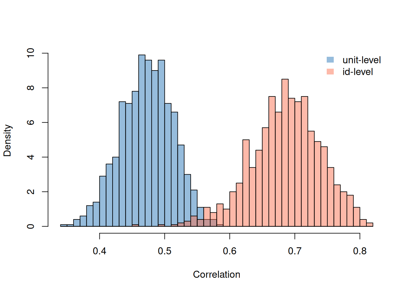
Figure 7.4: Posterior distributions for the correlations between log(\(\texttt{bili}\)) and the presence of ascites (on the latent scale).
In the model with two Gaussian responses we also thought about the association between the two traits in terms of regression. If we follow the same recipe for the Bernoulii response (\(\texttt{ascites}\)) regressed on the Gaussian response (log(\(\texttt{bili}\))) we end up with regression coefficients had we fitted log(\(\texttt{bili}\)) as a predictor and also the true expected log(\(\texttt{bili}\)) of each patient (which of course we don’t know, but constitute the \(\texttt{id}\) effects for that trait). The change in the risk of \(\texttt{acites}\) when increasing a patient’s log(\(\texttt{bili}\)) by one unit is greater than the difference in risk between two patient’s that on average differ in log(\(\texttt{bili}\)) by one unit (Figure 7.5).
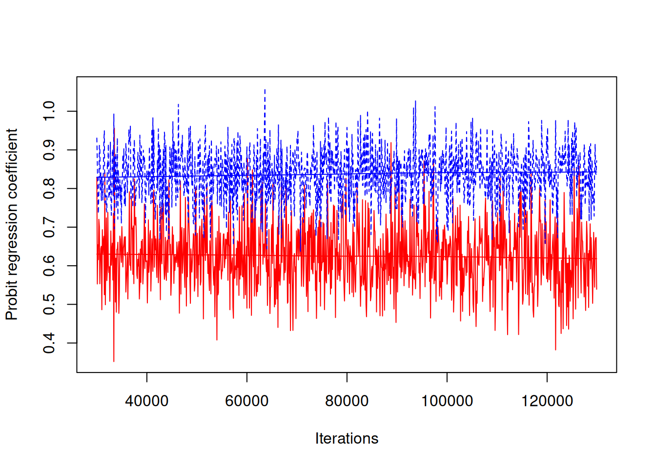
Figure 7.5: MCMC trace plot of the coefficient from a probit regression of ascites presence (\(\texttt{ascites}\)) on log serum concentration of bilirunbin (\(\texttt{bili}\)). The red and blue traces are from a model where the regression coefficient is estimated at two levels: within an individual (blue) and across individuals (red).
Note that this conclusion is opposite to the one you might draw from looking at the correlations. Why? The reason is that the proportion of variation that is within patients (Section 4.4) is quite different for the two traits: for log(\(\texttt{bili}\)) the posterior mean is 0.24 and for \(\texttt{acites}\) it is 0.54. The within-patient effects for log(\(\texttt{bili}\)) have proportionally little variation yet they still strongly correlate with the within-patient \(\texttt{acites}\) effects which have proportionally greater variation. We can also more formally assess whether the within-patient (\(\texttt{units}\)) regression is stronger than the between-patient regression:
preg.id<-m.pbc1$VCV[,"traitbili:traitascites.id"]/m.pbc1$VCV[,"traitbili:traitbili.id"]
preg.units<-m.pbc1$VCV[,"traitbili:traitascites.units"]/m.pbc1$VCV[,"traitbili:traitbili.units"]
HPDinterval(preg.units-preg.id)
## lower upper
## var1 -0.02286305 0.4562448
## attr(,"Probability")
## [1] 0.95The 95% credible interval overlaps zero, just.
If we consider the opposite regression - the Gaussian response (log(\(\texttt{bili}\))) on the Bernoulii response (\(\texttt{ascites}\)) things aren’t quite as straight forward. In a single response-model the actual presence or not of \(\texttt{ascites}\) would be fitted, yet in the multi response-model the association is at the level of the latent variable. As noted above for car accidents and insurance payouts, there is an important distinction between measuring an association directly on the data scale versus the latent scale. However, when Bernoulli models are conceptualised in terms of threshold models we can make this distinction disappear. If we designate the Gaussian response as \(y\) and the Bernoulli response as \(x\) (0 or 1) with associated latent variable \(l\), we can calculate the two expectations
\[E[y|x=1]=E[y | l>0]\]
and
\[E[y|x=0]=E[y | l<0]\]
The difference between these expectations is the coefficient you would obtain by fitting the Bernoulli variable (\(\texttt{ascites}\)) as a predictor in a model for the Gaussian response (log(\(\texttt{bili}\))). The difference is given by
\[E[y|x=1]-E[y|x=0]=\frac{f_N(\alpha)\sigma^2_{y,l}}{F_N(\alpha)(1-F_N(\alpha))\sigma_{l}}\]
where \(f_N\) and \(F_N\) are the density and cumulative density functions for the unit normal, and \(\alpha = \mu_l/\sigma_{l}\)35.
We can visualise what we have done. Figure 7.6 plots the 95% prediction interval for the latent variable associated with \(\texttt{ascites}\) presence (x-axis) and log(\(\texttt{bili}\)) (y-axis) assuming the mean is at the central black point (this is the posterior mean prediction for the data). Conditioning on the posterior mean estimates of \({\bf V}_{\texttt{id}}\) and \({\bf V}_{\texttt{units}}\), the predictive distribution is multivariate normal with covariance matrix \({\bf V}_{\texttt{id}}+{\bf V}_{\texttt{units}}\) and so the 95% prediction interval is an ellipse. When the latent variable exceeds zero (vertical dashed line) the \(y=1\) (\(\texttt{ascites}\) is present). Consequently, the blue shaded area is the region of the predictive distribution for individuals with \(\texttt{ascites}\) and the white region of the ellipse is for individuals without \(\texttt{ascites}\). The expectation of \(log(\texttt{bili})\) for these two groups are plotted as arrows.
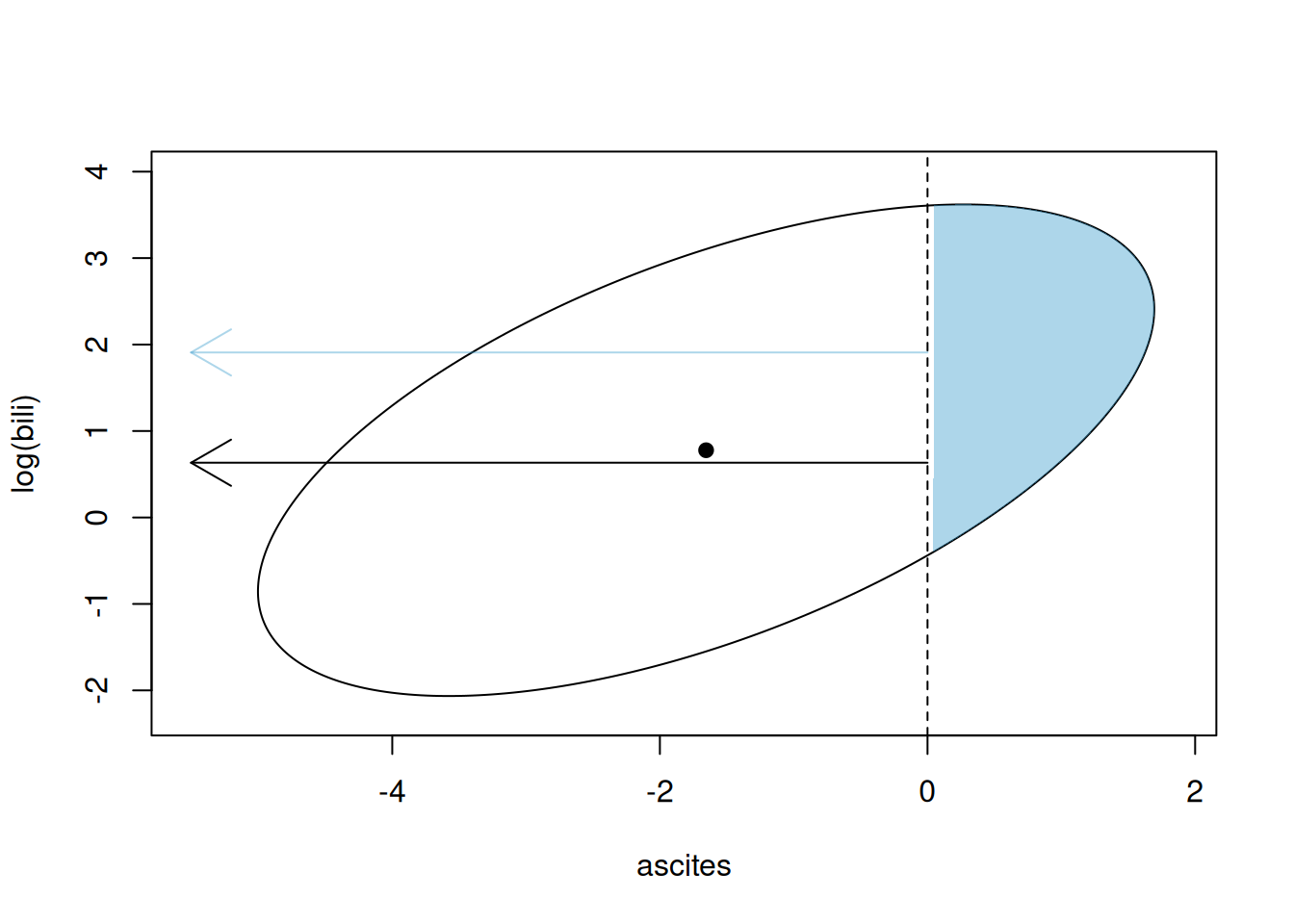
Figure 7.6: Representation of a Gaussian (\(log(\texttt{bili})\)) and Bernoulli (\(\texttt{ascites}\)) multi-response model. The ellipse is the 95% prediction interval for the Gaussian trait and the Bernoulli latent variable (on the probit scale). Observations to the right of the threshold (vertical dashed line) are successes and have \(\texttt{ascites}\) and those to the left do not. The means of the Gaussian variable in these two groups are plotted as arrows.
We can also plot the MCMC trace of the difference, and we can see that the difference is large and certainly not zero.
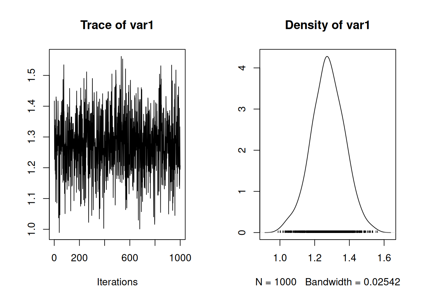
Figure 7.7: MCMC trace plot of the regression coefficient of log serum concentration of bilirunbin (\(\texttt{bili}\)) on ascites presence (\(\texttt{ascites}\)) as obtained from a multi-response model.
7.2.2 All Bernoulli
We can also consider a bivariate model of the two Bernoulli variables \(\texttt{ascites}\) and \(\texttt{hepato}\). The model set-up is almost identical, although we need to add the constraint that the residual variances of both traits are not identifiable in the likelihood but the residual correlation is: we need o restrict the residual covariance matrix to a residual correlation matrix. Replacing the \(\texttt{us}\) variance structure with \(\texttt{corg}\) achieves this. The prior specification only requires a degree-belief parameter \(\texttt{nu}\) which results in a beta distribution for each correlation with shape and scale equal to \((\texttt{nu}-k+1)/2\). Since \(k=2\), I set \(\texttt{nu}=3\) which results in a flat prior for the correlation. Note that specifying the marginal prior F(2,1000) for the (co)variance matrix of \(\texttt{id}\) effects also results in \(\texttt{nu}=3\) (See Section 5.3.2).
prior.pbc2<-list(R=list(V=diag(2),nu=3), G=F(2,1000))

m.pbc2<-MCMCglmm(cbind(hepato, ascites)~trait-1+trait:(age+sex), random=~us(trait):id, rcov=~corg(trait):units, data=pbcseq, family=c("threshold", "threshold"), prior=prior.pbc2, longer=10)
On the latent scale we see a reasonably strong correlation between the two outcomes:
##
##  Iterations = 30001:129901
##  Thinning interval  = 100
##  Sample size  = 1000
##
##  DIC:
##
##  G-structure:  ~us(trait):id
##
##                              post.mean l-95% CI u-95% CI eff.samp
## traithepato:traithepato.id      1.8985   1.3595    2.526     1000
## traitascites:traithepato.id     0.9391   0.6284    1.311     1000
## traithepato:traitascites.id     0.9391   0.6284    1.311     1000
## traitascites:traitascites.id    1.0110   0.6128    1.457     1000
##
##  R-structure:  ~corg(trait):units
##
##                                 post.mean l-95% CI u-95% CI eff.samp
## traithepato:traithepato.units      1.0000  1.00000   1.0000      0.0
## traitascites:traithepato.units     0.2394  0.07852   0.4175    903.7
## traithepato:traitascites.units     0.2394  0.07852   0.4175    903.7
## traitascites:traitascites.units    1.0000  1.00000   1.0000      0.0
##
##  Location effects: cbind(hepato, ascites) ~ trait - 1 + trait:(age + sex)
##
##                   post.mean  l-95% CI  u-95% CI eff.samp  pMCMC
## traithepato        0.402183 -0.792992  1.505713    872.8  0.478
## traitascites      -3.023644 -4.031956 -1.912948   1000.0 <0.001 ***
## traithepato:age    0.006753 -0.010265  0.024141    878.4  0.490
## traitascites:age   0.023952  0.006669  0.038642   1000.0 <0.001 ***
## traithepato:sexf  -0.580279 -1.153023  0.015449   1000.0  0.056 .
## traitascites:sexf  0.109574 -0.382191  0.659287   1000.0  0.720
## ---
## Signif. codes:  0 '***' 0.001 '**' 0.01 '*' 0.05 '.' 0.1 ' ' 1
If we wish, we can also characterise the relationship in terms of a contingency table. The model defines a multivariate normal distribution of latent variables around the fixed-effect prediction, and the probability of falling in any of the four quadrants defined by the origin can be calculated. We can imagine a population of individuals all of which have the same expected latent variables (the weighted average of the male and female means at the average age, where the weights are the frequencies of males and females in the data frame):
mu<-c(0,0)
nobs<-nrow(pbcseq) # number of obseravtions

mu[1]<-mean(predict(m.pbc2, type="terms")[1:nobs])
# predicted mean for hepato latent variable

mu[2]<-mean(predict(m.pbc2, type="terms")[nobs+1:nobs])
# predicted mean for ascites latent variable
Around these means the latent variables for a particular individual at a particular time (as a vector are) \({\bf u}_i+{\bf e}_{ij}\). These vectors are a drawn from a multivariate normal with zero mean and (co)variance \({\bf V}_{\texttt{id}}+{\bf V}_{\texttt{units}}\):
Figure 7.8 gives a visual representation of this distribution, and the quadrants that correspond to different outcomes.
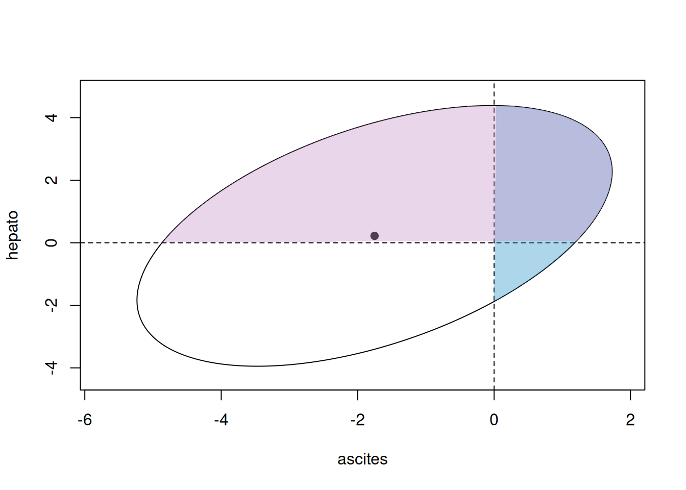
Figure 7.8: Representation of a bivariate Bernoulli model. The solid point represents the means of the two Bernoulli latent variables and the ellipse is the 95% prediction interval for the latent variables. The pair of latent variable lie in one of the four quadrants corresponding to the observed outcome (white: hepato=0 and ascites=0, pink: 1/0, blue: 0/1 and purple: 1/1).
The raw contingency table for the data is:
##       ascites
## hepato          0          1
##      0 0.49016481 0.01594896
##      1 0.41998937 0.07389686
The \(\texttt{pmnorm}\) function in the package \(\texttt{mnorm}\) calculates the cumulative density function for the multivariate normal, and we can use this to calculate the four probabilities. I’ve done this in a rather long winded way so that the code could be extended to ordinal data that falls into more than two categories (Section 3.7):
n<-2
m<-2
P<-matrix(NA, n, m)

thresh1<-c(-Inf, 0, Inf)
thresh2<-c(-Inf, 0, Inf)

for(i in 1:n){
    for(j in 1:m){
        lower<-c(thresh1[i], thresh2[j])
        upper<-c(thresh1[i+1], thresh2[j+1])
        P[i,j]<-mnorm::pmnorm(lower, upper, mean = mu, sigma = V)$prob
    }
}
We don’t expect the predicted probabilities to perfectly match what is observed since the data are unbalanced (individuals vary in how many times they are observed) and individuals vary in their sex and age but our prediction is for a population of individuals that are in some way average. Nevertheless, the predicted probabilities are close:
##           [,1]       [,2]
## [1,] 0.4321614 0.01520272
## [2,] 0.4589253 0.09371065
7.3 Wide versus Long Format
In the multi-response models we have fitted so far, all responses have been observed for every unit of observation. For example, there were no cases where a patient was assessed for \(\texttt{ascites}\) but \(\texttt{bili}\) was not measured. If there had been missing observations, these could have been recorded as \(\texttt{NA}\) and \(\texttt{MCMCglmm}\) will treat them as unknown observations to be sampled and averaged over. If the amount of missingness is low then this is generally not an issue. However, if there is a lot of missing data then updating the missing observations can be slow and result in poor mixing. In these cases it is usually best to store the data in long-format and remove the missing values 36. When fitting multi-response models to long-format data it needs to be in a format shown in Equation (7.1). There needs to be two columns in the data-frame: \(\texttt{family}\) specifying the distribution for each observation and \(\texttt{trait}\) which has factors indexing the observation type. In such cases the \(\texttt{family}\) argument to \(\texttt{family}\) should be \(\texttt{NULL}\).
In the next section we will fit a bivariate model to log(\(\texttt{bili}\)) and the categorical variable \(\texttt{status}\). \(\texttt{status}\) has three levels indicating whether the final outcome for the patient was censored (0) had a liver transplant (1) or died (2). Let’s reshape the data and add the necessary columns:
pbcseq_long <- tidyr::pivot_longer(pbcseq,
  cols      = c(status, bili),
  values_to = "y",
  names_to = "trait",
  cols_vary = "slowest")
# merge status and bili columns into a single column: y
# trait is the column indicating if y belongs to status or bili

pbcseq_long$trait<-as.factor(pbcseq_long$trait)

pbcseq_long$family <- dplyr::recode(pbcseq_long$trait, bili = "gaussian", status = "threshold")
# family specifies the distribution type for the two sets of observations.
7.4 Covariances between random and residual terms (\(\texttt{covu}\))
In the previous section we generated a long-format data-frame \(\texttt{pbcseq_long}\) with the response variable \(\texttt{y}\) being associated with two traits: \(\texttt{status}\) with three levels and then the continuous variable \(\texttt{bili}\). In reality, \(\texttt{status}\) is not a repeat-measure trait, it is the final outcome (censored, transplant or dead) duplicated across all of the patients records. Consequently we should only retain a single record:
remove<-with(pbcseq_long, duplicated(id) & trait=="status")
# cols_vary = "slowest" in pivot_longer means status records are followed by bili
# Then, `remove` is TRUE for all status observations except the first for each id.

pbcseq_long<-pbcseq_long[-which(remove),]

# rows of data-frame for first patient
subset(pbcseq_long[,c("y", "trait", "family", "id")], id==1)
## # A tibble: 3 × 4
## y trait family id
## <dbl> <fct> <fct> <int>
## 1 2 status threshold 1
## 2 14.5 bili gaussian 1
## 3 21.3 bili gaussian 1In addition lets log transform \(\texttt{bili}\) and turn \(\texttt{status}\) into a 2-level outcome dead (1) or not (0):
pbcseq_long <- pbcseq_long %>% mutate(y = if_else(trait == "bili", log(y),y))
pbcseq_long <- pbcseq_long %>% mutate(y = if_else(trait == "status", as.numeric(y == 2),y))
If we wish to model death and \(\texttt{bili}\) simultaneously, the Bernoulli-Gaussian model covered in Section 7.2.1 seems appropriate. However, since we only have a single-record of \(\texttt{status}\) for each patient, it doesn’t make sense to fit \(\texttt{id}\) effects for \(\texttt{status}\) as they are not identifiable from the \(\texttt{unit}\) effects (which themselves have non-identifiable variance because \(\texttt{status}\) is Bernoulli). However, \(\texttt{bili}\) is repeat-measure and so it does make sense to fit \(\texttt{id}\) effects for this traits. In addition, allowing the \(\texttt{id}\) effects for \(\texttt{bili}\) to be correlated with the \(\texttt{unit}\) effects of \(\texttt{status}\) also seems reasonable - perhaps the long-term concentration of bilirunbin dictates whether a patient will live or not. In Section 5.2 we covered ways in which we could link two (or more) sets of random effects and estimate their covariance matrix. Here, we need to link a set of random effects with a set of residuals. \(\texttt{MCMCglmm}\) allows the set of random effects appearing in the final random term of the random specification to be correlated with the set of residuals appearing in the first residual term of the rcov specification. The linking is specified by adding a covu=TRUE to the prior specification for the first residual term.
prior.pbc_long<-list(R=list(R1=list(V=diag(2),nu=3, covu=TRUE, fix=2),
                            R2=IW(1, 0.002)))

m.pbc_long<-MCMCglmm(y~trait-1+at.level(trait, "bili"):(age+sex)-1+at.level(trait, "status"):sex,
                random=~us(at.level(trait, "bili")):id,
                rcov=~us(at.level(trait, "status")):id+us(at.level(trait, "bili")):units,
                data=pbcseq_long, family=NULL, prior=prior.pbc_long)
The model specification requires a bit of unpacking. trait-1 fits intercepts for both traits. at.level(trait, "bili"):(age+sex) fits an age effect and a sex effect to (log) \(\texttt{bili}\) and at.level(trait, "status"):sex fits a sex effect for \(\texttt{status}\). random=~us(at.level(trait, "bili")):id fits \(\texttt{id}\) effects for \(\texttt{bili}\). This works because at.level(trait, "bili") defines a vector of zero’s (if \(\texttt{trait}=\texttt{status}\)) and one’s (if \(\texttt{trait}=\texttt{bili}\)) for which random slopes are defined (see Chapter 6). Consequently, when \(\texttt{trait}=\texttt{status}\) the model is \(0\times u =0\) and when \(\texttt{trait}=\texttt{bili}\) the model is \(1\times u =u\), where \(u\) is the \(\texttt{id}\) effect. Similarly, the first part of the residual specification us(at.level(trait, "status")):id defines a complementary set of residuals for \(\texttt{status}\). This works because for \(\texttt{status}\) there is only one observation per level of \(\texttt{id}\) and so the specification satisfies the condition for a residual: the effect must be unique to an observation. Using us(at.level(trait, "status")):units would also have satisfied this condition, but the levels in the residual specification need to correspond to those in the random term for them to be linked, hence \(\texttt{id}\) was used rather than \(\texttt{units}\). Finally, we have a second residual component that defines the residuals for \(\texttt{bili}\): us(at.level(trait, "bili")):units. The prior for the first residual term (\(\texttt{R1}\)) contains the argument covu=TRUE indicating that covariances between the set of residuals and the set of random effects defined by the final random term are present. The prior for the resulting (\(2\times 2\)) covariance matrix is also specified here and the prior for the final random term (the only random term in this model) is omitted. Note that the variance structure is that specified by the residual term (\(\texttt{us}\) in this instance). We have fixed the second variance in this covariance matrix to one, since these are the \(\texttt{unit}\) effects for a Bernoulli trait and so the variance isn’t identified. Using \(\texttt{nu=3}\) places a flat prior on the correlation (Section 5.3.2) but the marginal prior for the variance of the \(\texttt{id}\) effects on \(\texttt{bili}\) is inverse-Wishart with \(\texttt{V=1.5}\) and \(\texttt{nu=2}\). Not ideal, but it is not possible to use parameter-expansion (Section 4.6) with \(\texttt{covu}\) structures.
##
##  Iterations = 3001:12991
##  Thinning interval  = 10
##  Sample size  = 1000
##
##  DIC: 3890.091
##
##  G-structure:  ~us(at.level(trait, "bili")):id
##
##  G-R structure below
##
##  R-structure:  ~us(at.level(trait, "status")):id
##
##                                                           post.mean l-95% CI
## at.level(trait, "bili").id:at.level(trait, "bili").id        1.0526   0.8665
## at.level(trait, "status").id:at.level(trait, "bili").id      0.6843   0.5586
## at.level(trait, "bili").id:at.level(trait, "status").id      0.6843   0.5586
## at.level(trait, "status").id:at.level(trait, "status").id    1.0000   1.0000
##                                                           u-95% CI eff.samp
## at.level(trait, "bili").id:at.level(trait, "bili").id       1.2296   1000.0
## at.level(trait, "status").id:at.level(trait, "bili").id     0.8056    900.8
## at.level(trait, "bili").id:at.level(trait, "status").id     0.8056    900.8
## at.level(trait, "status").id:at.level(trait, "status").id   1.0000      0.0
##
##                ~us(at.level(trait, "bili")):units
##
##                                                       post.mean l-95% CI
## at.level(trait, "bili"):at.level(trait, "bili").units    0.3181   0.2966
##                                                       u-95% CI eff.samp
## at.level(trait, "bili"):at.level(trait, "bili").units   0.3392     1000
##
##  Location effects: y ~ trait - 1 + at.level(trait, "bili"):(age + sex) - 1 + at.level(trait, "status"):sex
##
##                                post.mean  l-95% CI  u-95% CI eff.samp  pMCMC
## traitbili                       2.200768  1.510415  2.858600   1000.0 <0.001
## traitstatus                    -0.202017 -0.363184 -0.060197    911.2  0.010
## at.level(trait, "bili"):age    -0.018561 -0.028616 -0.008165   1000.0 <0.001
## at.level(trait, "bili"):sexf   -0.560530 -0.974695 -0.201330   1000.0  0.002
## sexm:at.level(trait, "status")  0.717815  0.289289  1.185448   1000.0 <0.001
##
## traitbili                      ***
## traitstatus                    **
## at.level(trait, "bili"):age    ***
## at.level(trait, "bili"):sexf   **
## sexm:at.level(trait, "status") ***
## ---
## Signif. codes:  0 '***' 0.001 '**' 0.01 '*' 0.05 '.' 0.1 ' ' 1
There is a strong positive association between the expected long-term value of (log) \(\texttt{bili}\) and whether a patient dies before the end of the study. Figure 7.9 shows the posterior distribution for the correlation in \(\texttt{id}\) effects.
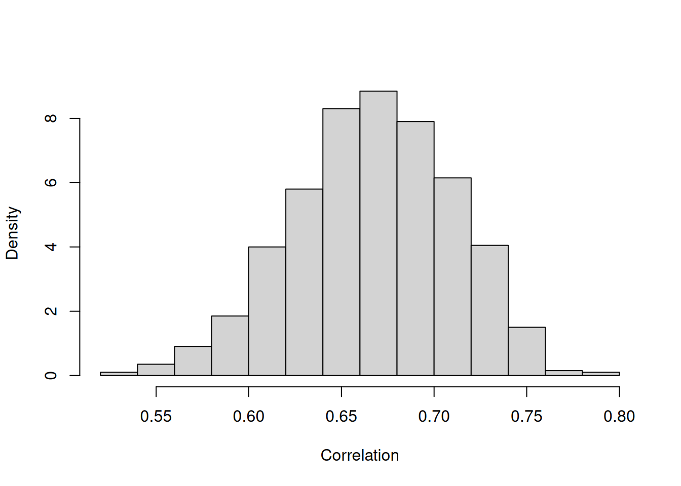
Figure 7.9: Posterior distribution of the correlation between patient effects on (log) \(\texttt{bili}\) and residual \(\texttt{status}\) (death) from model \(\texttt{m.pbc_long}\).
A more usual way to fit this type of model is to use a single-response for death and simply fit the average of each patient’s (log) \(\texttt{bili}\) as a predictor.
pbcseq_status<-subset(pbcseq_long, trait=="status")
pbcseq_status$mean.bili<-with(pbcseq, tapply(log(bili), id, mean))[pbcseq_status$id]

m.pbc_status<-MCMCglmm(y~mean.bili, data=pbcseq_status, family=NULL, prior=list(R=list(V=1, fix=1)))
In Figure 7.10 the regression coefficient from the multi-response model (in black) is compared to that from the single-response model (in red) and we can see that the multi-response model gives a regression coefficient that is greater in magnitude37.
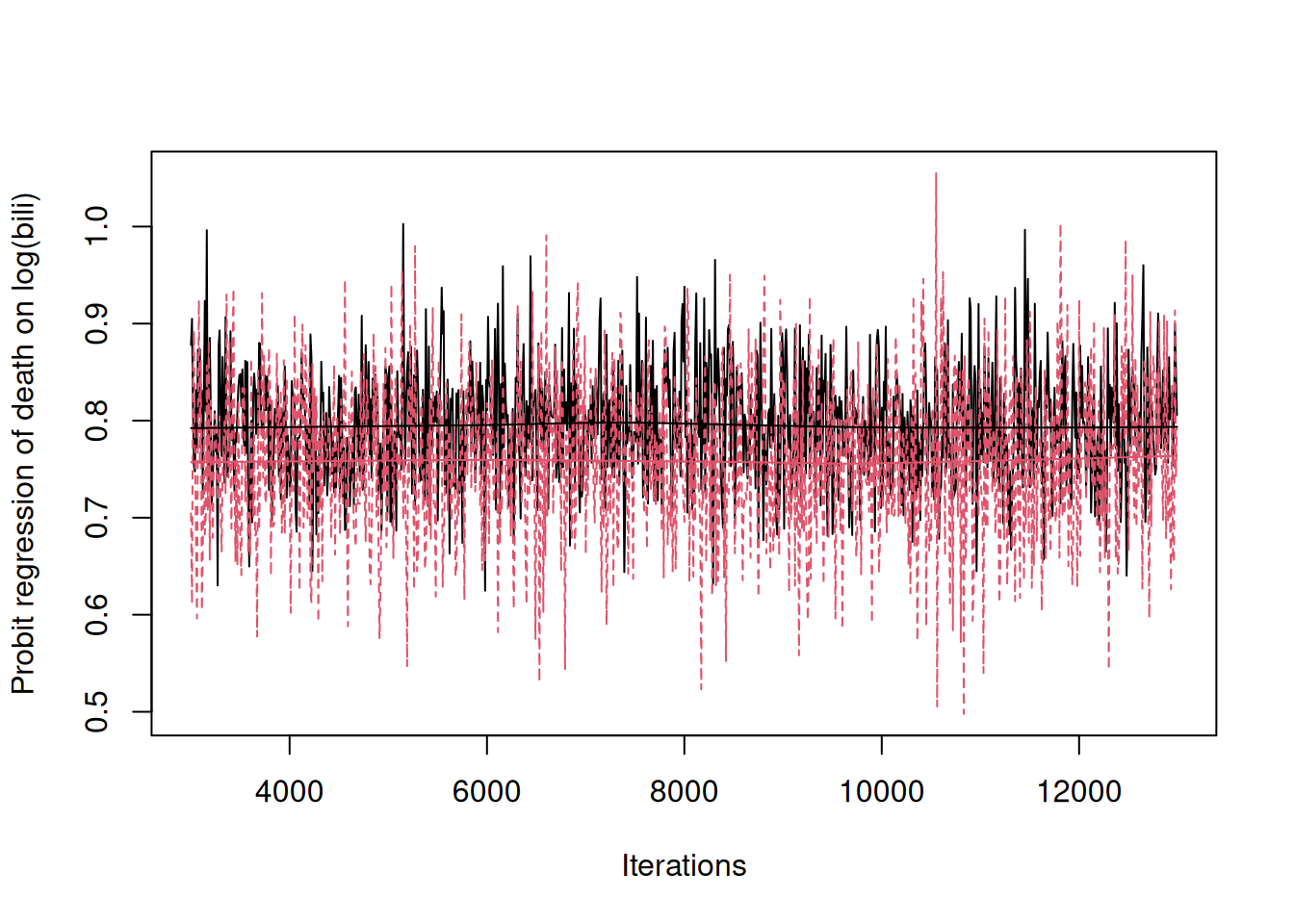
Figure 7.10: Posterior distributions for the probit regression of \(\texttt{status}\) (death) on a patient’s (log) \(\texttt{bili}\) value. The black trace is obtained from a multi-response model and the predictor is the expected value of log \(\texttt{bili}\) for each patient, whereas the red trace is obtained from a single-response model and the predictor is the sample mean of log \(\texttt{bili}\) for each patient.
The reason for this pattern is that the coefficient in the single-response model is attenuated because of the measurement error in the expected (log) \(\texttt{bili}\). If \(r\) is the correlation between the true value of a predictor and its measured value, we expect the regression using measured values to be equal to the regression obtained from the true values multiplied by \(r^2\) (see Chapter 9). However, the attenuation is small in this example because on average \(\texttt{bili}\) has been measured 6 times per patient and the within-patient variability is quite low - the intra-class correlation for log \(\texttt{bili}\) from the multi-response model is 0.77. Together the \(r^2\) is predicted to be 0.95 (\(\sigma^2_\texttt{bili.id}/(\sigma^2_\texttt{bili.id}+\sigma^2_\texttt{bili.units}/6)\)) - almost identical to the attenuation seen. In addition to dealing with the attenuation, the multi-response model also makes more efficient use of the data when the design is unbalanced (some patients only have a single measurement whereas others have up to 16) and the posterior standard deviation of the regression coefficient is 0.06 from the multi-response model but 0.08 from the standard single response model.
7.5 Scaled linear predictors: \(\texttt{theta_scale}\)
In the previous sections of this Chapter we’ve often thought about multi-response models in terms of regression. In some cases, the regression coefficient was different at different levels. For example, in Section 7.2.1 the regression within patients differed from the regression across patients. In other cases, the regression coefficient was only fitted for specific levels. For example, in Section 7.4 the regression was only fitted across patients not within. Although we parameterised the model in terms of unstructured covariance matrices (\(\texttt{us}\)) we could have fitted the same model parameterised in terms of regression coefficients and innovation variances using antedependence structures (see Section 6.5). Sometimes, however, we would like a model where the regression is held constant across two or more levels but is allowed to be different (or zero) at others. The \(\texttt{theta_scale}\) argument in \(\texttt{MCMCglmm}\) allows two sets of parameters to be fitted that differ by a common scaling factor. For example, we may have two vectors of random effects \(\{{\bf u}_1 {\bf u}_2\}\) that appear in the linear predictor of one set of observations and would like to fit the effects \(\{\theta_s{\bf u}_1 \theta_s{\bf u}_2\}\) for another set of observations. By fitting the first set of effects for one trait (the predictor) and the second set of effects to the other trait (the response) we can hold the regression constant (\(\theta_s\)) at the two levels defined by the random effects.
7.6 Multinomial Models
In the previous sections of this chapter we covered multi-response models where each response comes from a single parameter distribution. \(\texttt{MCMCglmm}\) also allows some distributions that are multi-parameter such as the multinomial and a range of zero-modified distributions. The syntax for fitting these models is similar to that for multi-response models with \(\texttt{trait}\) indexing the different parameters of the distribution and \(\texttt{units}\) indexing the observation.
We will start with multinomial models where the response is the number of counts in two or more nominal categories. When the number of categories is two we have the binomial which was covered in Section 3.6. In binomial models we condition on the total number of counts and the model is parameterised in terms of the probability of success, with failure being the base-line category. In multinomial models we also condition on the total number of counts and model the probability of belonging to each category compared to a base-line category. In both cases, it makes sense that the model is parameterised in terms of \(K-1\) comparisons since if we know \(K-1\) probabilities the final probability is known since the sum of all probabilities must equal one. As with binomial models, the number in each category can be passed as columns using cbind and then the base-line category is that associated with the final column. Alternatively, if the total number of counts is one, the response can be passed as a single vector of categories for each observation and then the base-line category is the first factor level of the response. In both cases, a logit-link is used.
To explore multinomial models we will analyse data collected by the Alaska Science Center on the prey items of seabirds breeding on Middleton Island in the Gulf of Alaska - see here. We will restrict ourselves to data obtained on the chicks of the wonderful Tufted Puffin:
##   year month Capelin Herring Pollock SandLance Other
## 1 1978   Jul       0       0       0         1     0
## 2 1978   Aug       0       0       0         1     0
## 3 1978   Aug       0       0       0         6     0
## 4 1978   Aug       0       0       0         1     0
## 5 1978   Aug       0       0       0         1     0
## 6 1978   Aug       0       0       0         1     0
Each row corresponds to one of 565 samples with their collection year and month recorded. The following four columns are the number of Capelin (\(\texttt{Capelin}\)), Pacific herring (\(\texttt{Herring}\)), Walleye pollock (\(\texttt{Pollock}\)) and Pacific sand lance (\(\texttt{SandLance}\)) in each sample. An additional 40 prey taxa were also recorded and their combined counts per sample are in the final column (\(\texttt{Other}\)). Figure 7.11 plots the number of prey items for 150 random samples.
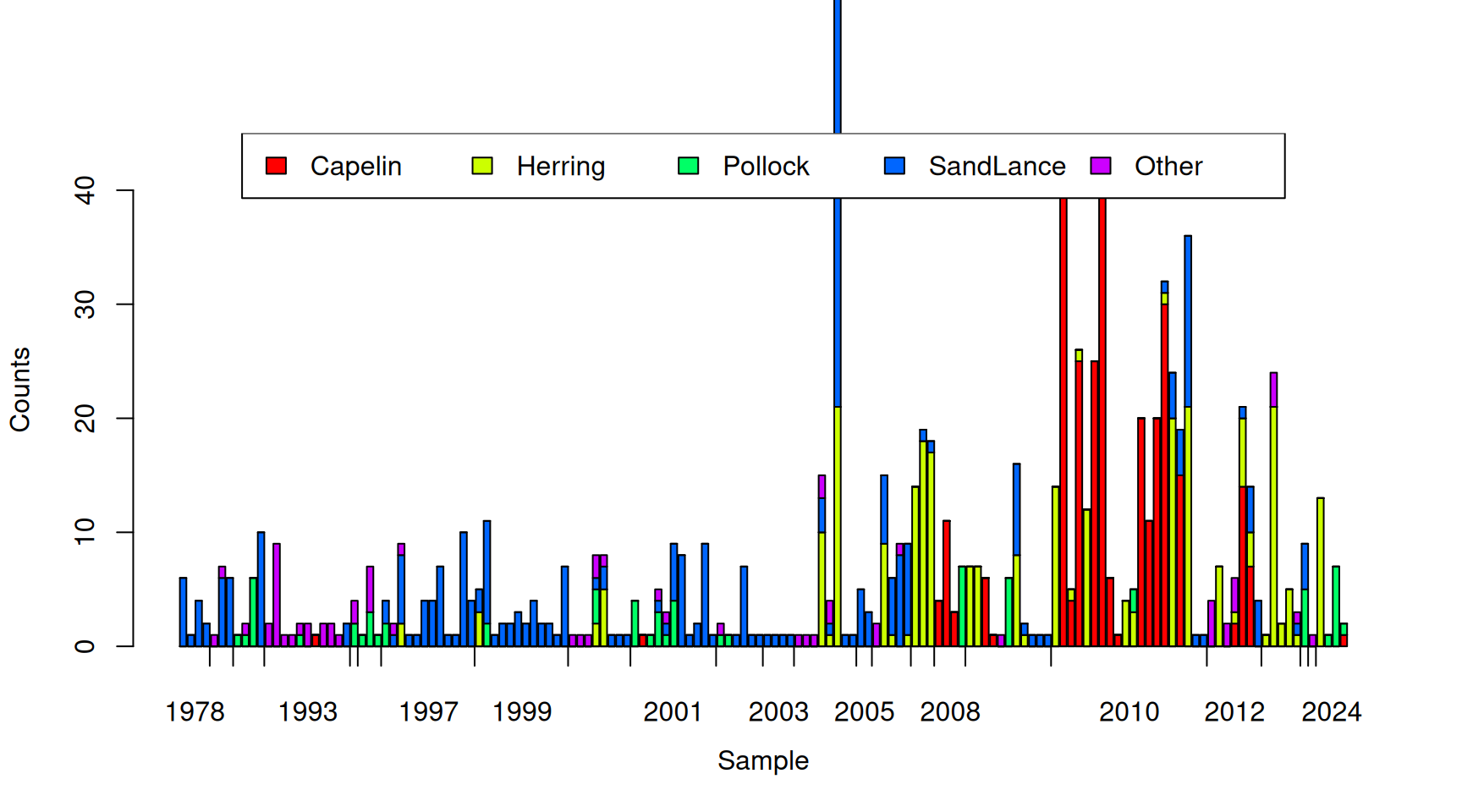
Figure 7.11: Number of prey items of different types in 150 randomly selected samples from Tufted Puffin chicks. The tick-marks on the x-axis delimit samples taken in the same year, and within years, samples are ordered by the proportion of prey items that are Pacific sand lance.
In terms of numbers, Capelin and the Pacific sand lance are the most common prey items, with ‘Other’ being the rarest
##   Capelin   Herring   Pollock SandLance     Other
## 1.7238938 1.1522124 0.6141593 1.6300885 0.5150442
However, there is tremendous variation in the total number of prey items per sample and it looks as if those samples with many prey items are dominated by Capelin. The multinomial ignores (conditions on) the total number of prey items and essentially works with the proportions of each prey item, as shown in Figure 7.12 for the 150 random samples.
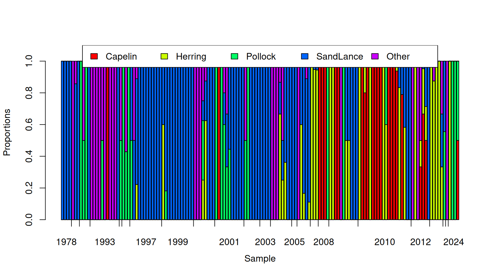
Figure 7.12: Proportion of prey items that are of each type in 150 randomly selected samples from Tufted Puffin chicks. The tick-marks on the x-axis delimit samples taken in the same year, and within years, samples are ordered by the proportion of prey items that are Pacific sand lance.
Once we control for the total number of prey items we see that Capelin actually makes up the lowest proportion of the diet and Pacific sand lance dominates:
##   Capelin   Herring   Pollock SandLance     Other
## 0.1200594 0.1316400 0.1449124 0.4062647 0.1971235
It is also apparent from Figure 7.12 (and Figure 7.11) that samples from the same year seem to have very similar compositions. Although less obvious, it also looks like there will be overdispersion - even within years, samples seem to vary in composition more than you would expect from multinomial sampling alone. In Figure 7.13 I have sampled from the multinomial with the probabilities given above and the observed total number of prey items for each of the 150 samples plotted. It is clear that the simulated data are much less structured than the real data shown in Figure 7.12.
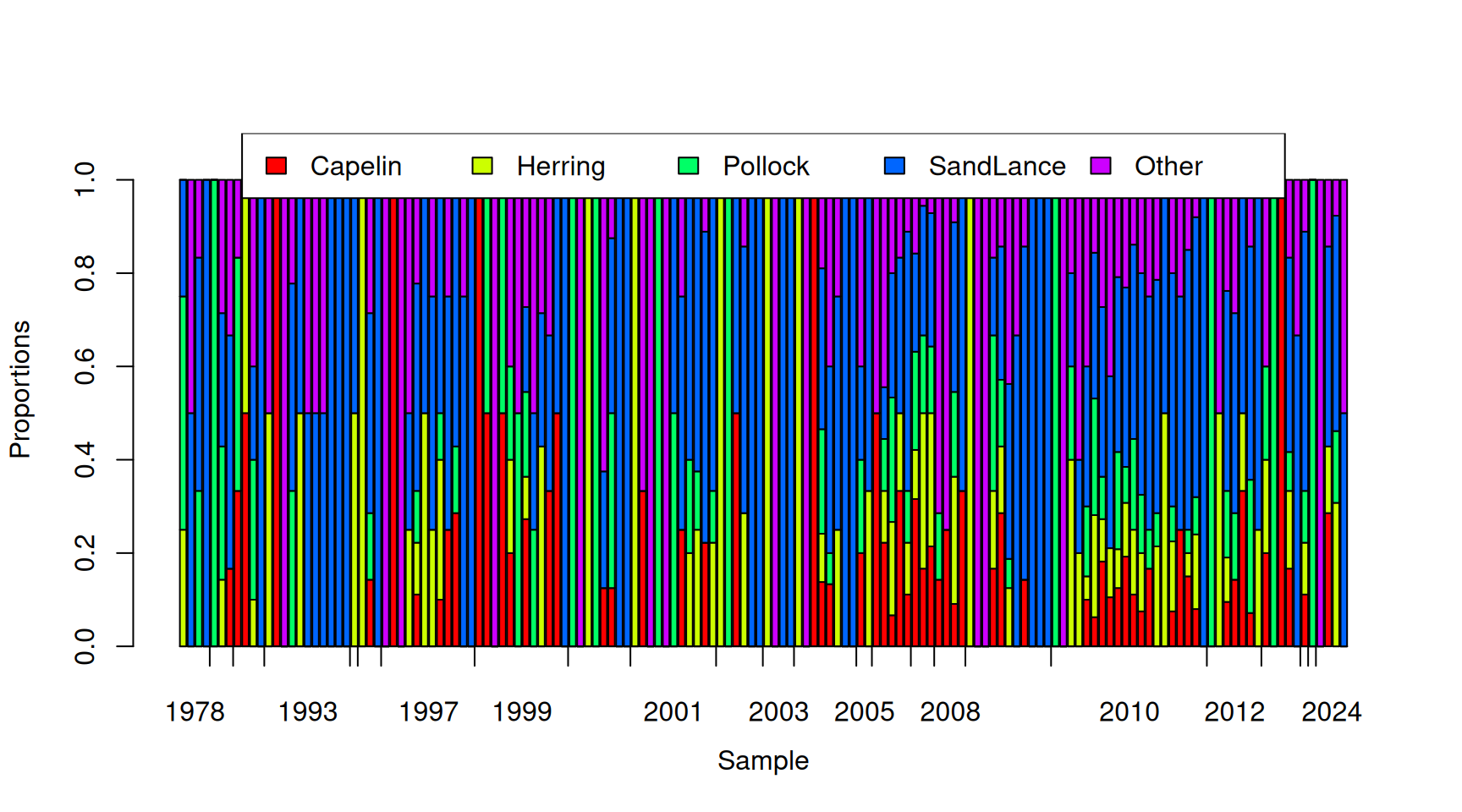
Figure 7.13: Simulated proportion of prey items that are of each type assuming that the probability of a prey item is constant over the samples. The tick-marks on the x-axis delimit samples taken in the same year, and within years, samples are ordered by the proportion of prey items that are Pacific sand lance.
Let’s fit a multinomial model to these data, using \(\texttt{Other}\) as the base-line category. We will also fit fully unstructured, \(4\times 4\), covariance matrices at the level of year and sample (\(\texttt{unit}\)):
prior.tufted<-list(R=IW(1, 2), G=F(2,1000))
m.tufted<-MCMCglmm(cbind(Capelin, Herring, Pollock, SandLance, Other)~trait-1, data=tufted_puffin, random=~us(trait):year, rcov=~us(trait):units, family="multinomial", longer=20, prior=prior.tufted, pr=TRUE)
With two \(4\times 4\) covariance matrices, the model summary is pretty overwhelming. To get a feel for the broad patterns, I have summarised the two matrices in terms of correlations (upper-triangle), variances (diagonals) and covariances (lower-triangle) in Table 7.1. The posterior means together with the 95% credible intervals (in square brackets) are reported.
| Capelin | Herring | Pollock | SandLance | |
|---|---|---|---|---|
| \({\bf V}_\texttt{year}\) | ||||
| Capelin | 73.70 [17.46-155.58] | 0.09 [-0.38-0.58] | 0.23 [-0.21-0.71] | -0.14 [-0.55-0.34] |
| Herring | 4.06 [-22.30-34.93] | 37.63 [9.17-82.47] | -0.16 [-0.55-0.33] | 0.36 [-0.03-0.73] |
| Pollock | 7.10 [-7.95-29.48] | -3.52 [-15.62-7.27] | 12.91 [3.65-25.38] | -0.23 [-0.62-0.20] |
| SandLance | -5.02 [-22.75-13.27] | 9.23 [-1.94-25.83] | -3.40 [-11.26-2.55] | 17.01 [6.12-30.69] |
| \({\bf V}_\texttt{units}\) | ||||
| Capelin | 65.79 [25.13-115.29] | -0.14 [-0.55-0.30] | -0.04 [-0.51-0.53] | -0.03 [-0.45-0.39] |
| Herring | -4.24 [-19.31-9.92] | 16.96 [8.44-26.08] | -0.00 [-0.49-0.44] | 0.68 [0.49-0.84] |
| Pollock | -0.42 [-9.44-9.01] | 0.10 [-3.53-4.33] | 4.33 [1.77-7.07] | 0.03 [-0.42-0.50] |
| SandLance | -0.77 [-15.71-13.58] | 11.25 [5.35-18.40] | 0.40 [-3.57-4.26] | 15.93 [8.95-24.26] |
There seems to be substantial variation, both between years and between samples, in the linear predictors for each prey item. Although credible intervals are wide, the generally pattern seems to be that the between year variation exceeds the between sample variation. Correlations between the linear predictors for different prey items also have wide credible intervals, but in general they seem fairly small. The exception to this is between the \(\texttt{Herring}\) and \(\texttt{SandLance}\) predictors, where the correlation is moderately positive, particularly at the level of samples (\(\texttt{units}\)).
Does the model fit the data? We can generate a draw from the posterior predictive distribution for the specific years sampled using the predict function and specifying \(\texttt{marginal=NULL}\):
This is a vector of counts of length \(n(K-1)\) where the first \(n\) values are the counts (in this example) for Capelin and the second set of \(n\) values are for Herring and so on. The counts for \(\texttt{Other}\) are not returned but can be obtained by taking the difference between the total number of counts for each observation and the sum of the counts across the other \(K-1\) categories. If we plot the quantiles of the observed number of counts against the quantiles of the posterior prediction for the number of counts we see a very strong 1:1 relationship (Figure 7.14).

Figure 7.14: qq-plot of prey item counts from a posterior predictive simulation of model \(\texttt{m.tufted}\) (x-axis) versus the empirical quantiles (y-axis).
However, this is rather misleading. The strong relationship may simply be driven by variation in the total number of counts per sample - something that is not modelled, but conditioned on. For this reason, I usually focus on the proportions when assessing the adequacy of the model. The qq-plot of the proportions shows a slightly noisier relationship, but still, it looks like the the marginal distribution of the data is captured well by the model (Figure 7.15).
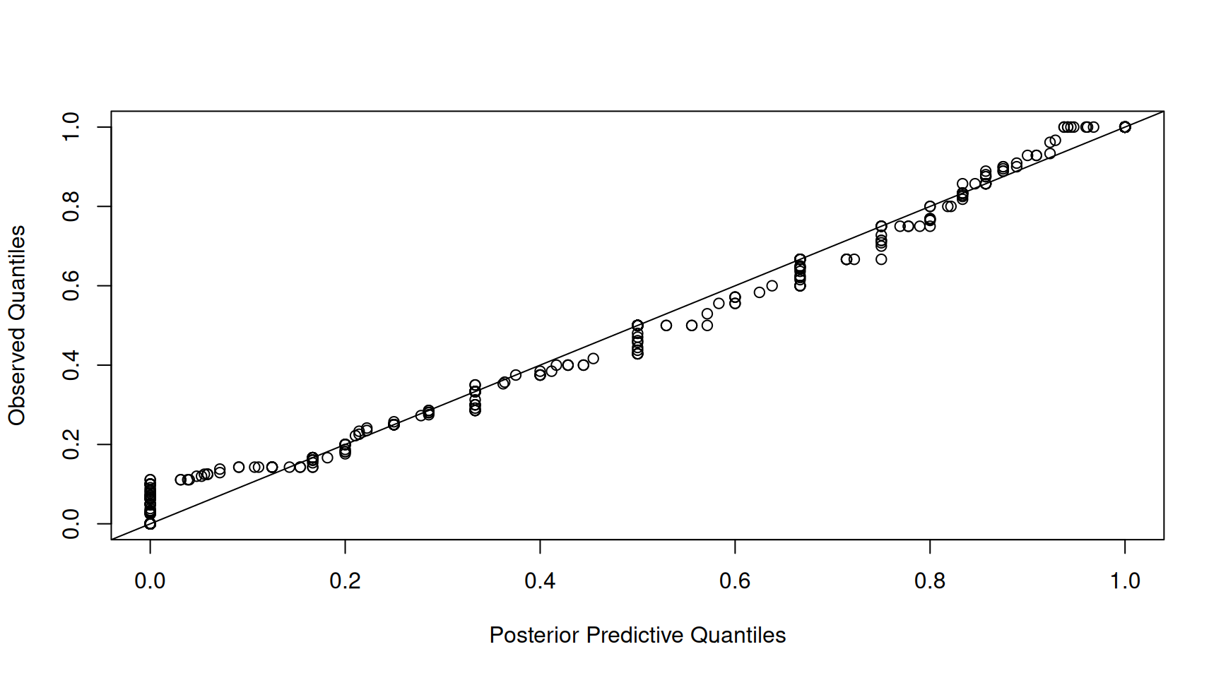
Figure 7.15: qq-plot of prey item proportions from a posterior predictive simulation of model \(\texttt{m.tufted}\) (x-axis) versus the empirical quantiles (y-axis).
While these qq-plots are good for assessing whether the model captures broad aspects of the data distribution, they don’t really provide insight as to whether the finer patterns have been captured well - for example, if changes in the composition of the samples over time has been adequately modelled. In Figure 7.16 I have plotted the proportion of each prey item for 150 random chicks as obtained from the posterior simulation (top) and compared it to the actual diet compositions (bottom). We can see, at least qualitatively, that the model seems to be picking up the structuring due to year rather well. Within years, we do not expect the posterior simulation to match the observation perfectly, since we are drawing a sample for a new chick within that year (the predict function always marginalises residual \(\texttt{unit}\) effects). However, if the model is doing a good job the distribution of compositions within years should look reasonable. Although hard to judge, there appears to be no major discrepancies - the model does predict that samples tend to be dominated by a single prey item even if the dominating prey item varies to some degree across samples within a year.
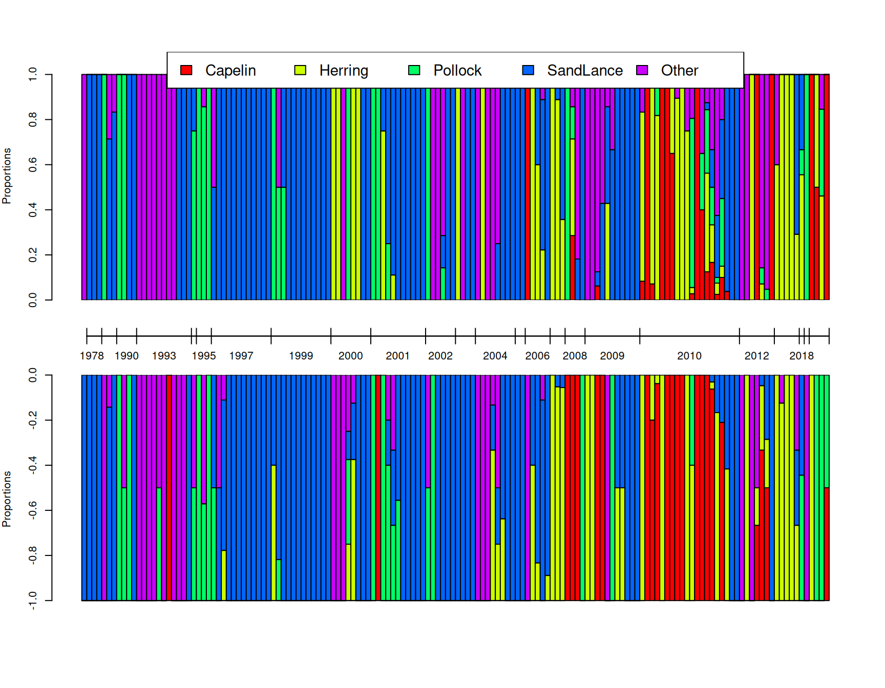
Figure 7.16: A posterior predictive simulation (top) using model \(\texttt{m.tufted}\) for the proportion of prey items that are of each type in 150 randomly selected samples. On the bottom are the observed proportion of prey items. The tick-marks on the x-axis delimit samples taken in the same year, and within years, samples are ordered by the proportion of prey items that are Pacific sand lance. Note that \(\texttt{unit}\) effects are marginalised in the posterior predictive simulation and so we do not expect an exact correspondence between samples: only the distributions within and across years should match.
While the pictures are pretty, we need to go beyond them to get a full understanding of what the model is telling us. With \(K=5\) categories we have \(K-1=4\) latent variables (traits) that are the log-odds ratio of observing a particular prey item versus the base-line prey item, in this case \(\texttt{Other}\). Abbreviating the prey types by their initial, the latent variables for sample \(i\) in year \(j\) are
\[ \begin{array}{rcl} l^{(\texttt{C-O})}_{ij} =& \textrm{log}\left(\frac{Pr(\texttt{C}_{ij})}{Pr(\texttt{O}_{ij})}\right)&= \beta^{(\texttt{C-O})}_0+u^{(\texttt{C-O})}_{j}+e^{(\texttt{C-O})}_{ij}\\ l^{(\texttt{H-O})}_{ij} =& \textrm{log}\left(\frac{Pr(\texttt{H-O}_{ij})}{Pr(\texttt{O}_{ij})}\right)&= \beta^{(\texttt{H-O})}_0+u^{(\texttt{H-O})}_{j}+e^{(\texttt{H-O})}_{ij}\\ l^{(\texttt{P-O})}_{ij} =& \textrm{log}\left(\frac{Pr(\texttt{P}_{ij})}{Pr(\texttt{O}_{ij})}\right)&= \beta^{(\texttt{P-O})}_0+u^{(\texttt{P-O})}_{j}+e^{(\texttt{P-O})}_{ij}\\ l^{(\texttt{S-O})}_{ij} =& \textrm{log}\left(\frac{Pr(\texttt{S}_{ij})}{Pr(\texttt{O}_{ij})}\right)&= \beta^{(\texttt{S-O})}_0+u^{(\texttt{S-O})}_{j}+e^{(\texttt{S-O})}_{ij}\\ \end{array} \]
where the \(\beta_0\) are trait-specific intercepts, the \(u\) are trait-specific year effects and and the \(e\) are trait-specific sample (\(\texttt{unit}\)) effects that capture overdispersion. The effects for each trait are really comparisons against the base-line category, \(\texttt{Other}\), and I have used a notation that makes this explicit, since it is easy to forget. Nevertheless, it needs to be kept in mind. For example, let’s imagine that Capelin and Herring appear in the diet completely independently of each other and so knowing there are many Capelin in a particular year is not informative about the abundance of Herring. It might then be tempting to assume that two sets of year effects, \(u^{(\texttt{C-O})}\) and \(u^{(\texttt{H-O})}\) are uncorrelated. However, they may be correlated through their shared dependence on \(\texttt{Other}\) prey items. To understand this, I often find it easier to think about the multinomial as a multivariate Poisson which is then followed by normalisation. The ratio of the probabilities, for example of Capelin versus \(\texttt{Other}\), is also equal to the ratio of expected counts:
\[\frac{Pr(\texttt{C}_{ij})}{Pr(\texttt{O}_{ij})} = \frac{n_{ij}Pr(\texttt{C}_{ij})}{n_{ij}Pr(\texttt{O}_{ij})}=\frac{E[n^{(\texttt{C})}_{ij}]}{E[n^{(\texttt{0})}_{ij}]}\]
where \(n_{ij}\) is the total number of counts across all categories: \(n_{ij}=n^{(\texttt{C})}_{ij}+n^{(\texttt{H})}_{ij}+n^{(\texttt{P})}_{ij}+n^{(\texttt{S})}_{ij}+n^{(\texttt{O})}_{ij}\). Sine a Poisson GLM with log-link involves linear models of the log expectation, we can interpret each parameter in the multinomial model as the difference in parameters from a bivariate Poisson model. For example, if we have log-linear models for the Capelin and \(\texttt{Other}\) counts:
\[ \textrm{log}\left(E[n^{(\texttt{C})}_{ij}]\right) = \beta^{(\texttt{C})}_0+u^{(\texttt{C})}_{j}+e^{(\texttt{C})}_{ij}\\ \]
\[ \textrm{log}\left(E[n^{(\texttt{O})}_{ij}]\right) = \beta^{(\texttt{O})}_0+u^{(\texttt{O})}_{j}+e^{(\texttt{O})}_{ij}\\ \]
then the parameters of the multinomial model are \(\beta^{(\texttt{C-O})}_0 = \beta^{(\texttt{C})}_0-\beta^{(\texttt{O})}_0\), \(u^{(\texttt{C-O})}_{j}=u^{(\texttt{C})}_{j}-u^{(\texttt{O})}_{j}\) and \(e^{(\texttt{C-O})}_{ij}=e^{(\texttt{C})}_{ij}-e^{(\texttt{O})}_{ij}\).
The assumption that the abundance of Capelin in a particular year is independent of the abundance of Herring implies that \(COV(u^{(\texttt{C})}, u^{(\texttt{H})})=0\). However, the covariance of the year effects in the multinomial is (for Capelin and Herring):
\[ \begin{array}{rl} COV(u^{(\texttt{C-O})}, u^{(\texttt{H-O})})=&COV(u^{(\texttt{C})}-u^{(\texttt{O})}, u^{(\texttt{H})}-u^{(\texttt{O})})& \\ =&COV(u^{(\texttt{C})}, u^{(\texttt{H})})-COV(u^{(\texttt{C})}, u^{(\texttt{O})})-COV(u^{(\texttt{H})}, u^{(\texttt{O})}) +VAR(u^{(\texttt{O})})& \\ \end{array} \]
and would remain non-zero even if \(COV(u^{(\texttt{C})}, u^{(\texttt{H})})=0\). If the abundances of Capelin, Herring and \(\texttt{Other}\) are all independent, the covariance simplifies to \(VAR(u^{(\texttt{O})})\) reflecting the shared dependence of the two log-odds on the base-line category, \(\texttt{Other}\). Similarly, the variance of year effects in the multinomial is (for Capelin):
\[ \begin{array}{rl} VAR(u^{(\texttt{C-O})})=&VAR(u^{(\texttt{C})})+VAR(u^{(\texttt{O})})-2COV(u^{(\texttt{C})}, u^{(\texttt{O})})\\ \end{array} \]
Even if the abundance of Capelin and \(\texttt{Other}\) are independent across years, the variance in the log-odds depends on the year variance of both categories: \(VAR(u^{(\texttt{C})})+VAR(u^{(\texttt{O})})\).
When we fitted multi-response models previously we naturally assumed that a diagonal covariance matrix somehow represents a null - the two traits are independent of each other. However, the above results suggest that we may need to modify our null when thinking about multinomial models. If we think that the log abundances of different prey items are independent across years but have the same yearly variation, then our null for the covariance matrix of multinomial year effects would have \(2\sigma^2_{u}\) along the diagonal and \(\sigma^2_{u}\) on the off-diagonals. Looking at the estimates when we fitted a fully unstructured covariance matrix for the year effects (Table 7.1) suggest this model may not perform that well. While the between-year variances have large credible intervals, and so a common variance of around 20 may not be too bad, a common covariance of 10 (correlation of 0.5) looks too large. Nevertheless, we can fit this model and assess the fit. We can represent the covariance structure of the year effects in this model as \({\bf V}_{\texttt{year}} = \sigma^2_{u}({\bf I}+{\bf J})\) where \({\bf I}\) and \({\bf J}\) are \(4\times 4\) identity and unit matrices, respectively38. To fit a year covariance matrix of this form we can use an \(\texttt{idv}\) variance structure with model formula trait+at.set(trait, 1:(K-1))39:
m.tuftedb<-MCMCglmm(cbind(Capelin, Herring, Pollock, SandLance, Other)~trait-1, data=tufted_puffin, random=~idv(~trait+at.set(trait, 1:4)):year, rcov=~us(trait):units, family="multinomial", longer=20, prior=prior.tufted, pr=TRUE)The posterior mean and 95% credible interval of \(\sigma^2_u\) is 13.19 [7.94-19.57]. In the fully unstructured model (\(\texttt{m.tufted}\)) the average of the four between-year variances halved was 17.66 and the average of the six between-year covariances was 2.55 (see Table 7.1). The estimate of \(\sigma^2_u\) can be seen as a compromise estimate of these ten parameters. To assess whether this simpler model does a good job at capturing the differences between years we can decide on a suitable metric and compare the metric calculated on the observed data with that calculated on posterior predictive simulations. One possible metric would be to calculate the mean proportions of Capelin, Herring, Pollock and Sand lance across samples for each year and then take the variance in these year means for each prey item or the correlation between year means for pairs of prey items. Relating this metric to the parameters of the model is not straight forward since the sample means for each year will, in part, reflect between sample variability, particularly in years where replication is low. In addition, the model works with log-probabilities, yet the described metric works with raw proportions since these are often zero and logging isn’t an option. Despite the metric’s limitations, I would still expect it to reveal major problems with the specified year effects.
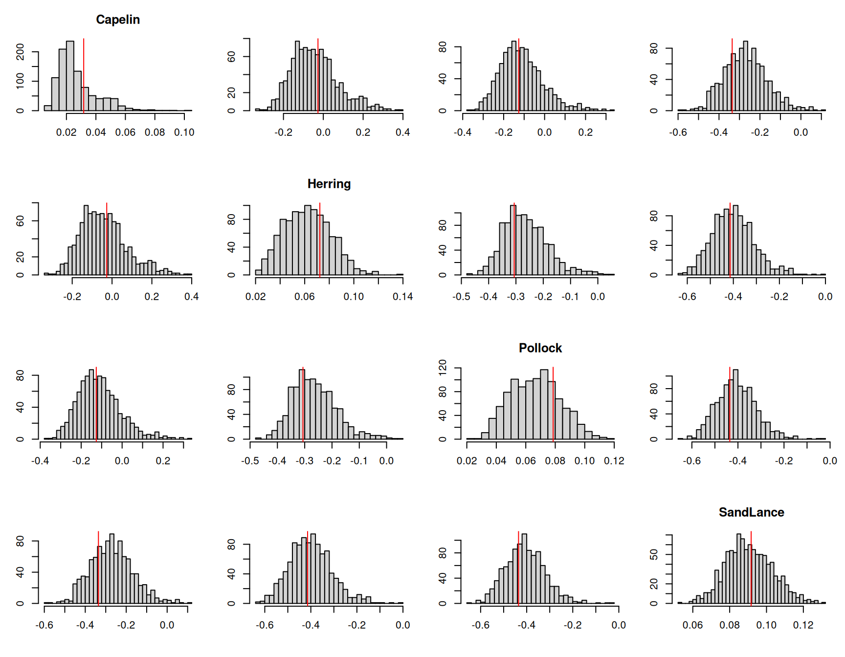
Figure 7.17: The mean proportion of each prey item across samples in a given year were calculated for one thousand posterior predictive simulations from model \(\texttt{m.tuftedb}\). This histograms represent the posterior predictive distributions for the variances of the yearly means (diagonal) or the correlations in yearly means between prey items. The red lines are the values calculated from the data.
The posterior predictive simulations suggest that the model is not too disastrous. The posterior distributions for the covariances are centred a little above the observed values, and the posterior distributions for the variances are concentrated a little below the observed values. Nevertheless, the discrepancies are not extreme, and even for Capelin, the posterior predictive distribution includes higher variances than that observed.
We can also fit a model which retains the assumption of independence but allows the amount of yearly variation in abundance to differ across categories. The (co)variance in multinomial year effects would then be \({\bf V}_{\texttt{year}} = {\bf D}+\sigma^2_{\texttt{O}}{\bf J}\) where \({\bf D}\) is a diagonal matrix with four variances to be estimated in addition to \(\sigma^2_{\texttt{O}}\). This can be achieved using the model structure idh(trait):year+year. The first term fits independent effects for each of the four traits but allows them to have different variances which can interpreted as \(VAR(u^{(\texttt{C})})\), \(VAR(u^{(\texttt{H})})\), \(VAR(u^{(\texttt{P})})\) and \(VAR(u^{(\texttt{S})})\) from the Poisson model. The second term fits a year effect common to all traits, which can interpreted as \(VAR(u^{(\texttt{O})})\) from the Poisson model.
m.tuftedc<-MCMCglmm(cbind(Capelin, Herring, Pollock, SandLance, Other)~trait-1, data=tufted_puffin, random=~idh(trait):year+year, rcov=~us(trait):units, family="multinomial", longer=20, prior=prior.tufted, pr=TRUE)The posterior means and 95% credible intervals for the year variances are displayed in table 7.2. Again, the credible intervals are wide and a common variance of around 20 may not be too bad for all categories except \(\texttt{Other}\). The yearly variance for \(\texttt{Other}\) is considerably smaller, which is to be expected since this represents the covariance between year effects in the fully unstructured model which were consistently less than half the variances. A reduced between-year variance for the \(\texttt{Other}\) category seems biologically reasonable: since this category lumps 40 prey items which are likely to show some degree of independence in their abundances across years.
| Posterior Mean | l-95% CI | u-95% CI | |
|---|---|---|---|
| Capelin | 58.98 | 11.34 | 134.65 |
| Herring | 28.10 | 7.70 | 57.05 |
| Pollock | 10.96 | 1.89 | 22.17 |
| SandLance | 14.21 | 3.70 | 26.65 |
| Other | 1.35 | 0.00 | 4.46 |
If we perform the same posterior predictive check that we did for the previous model we can see it does a good job (Figure 7.18).
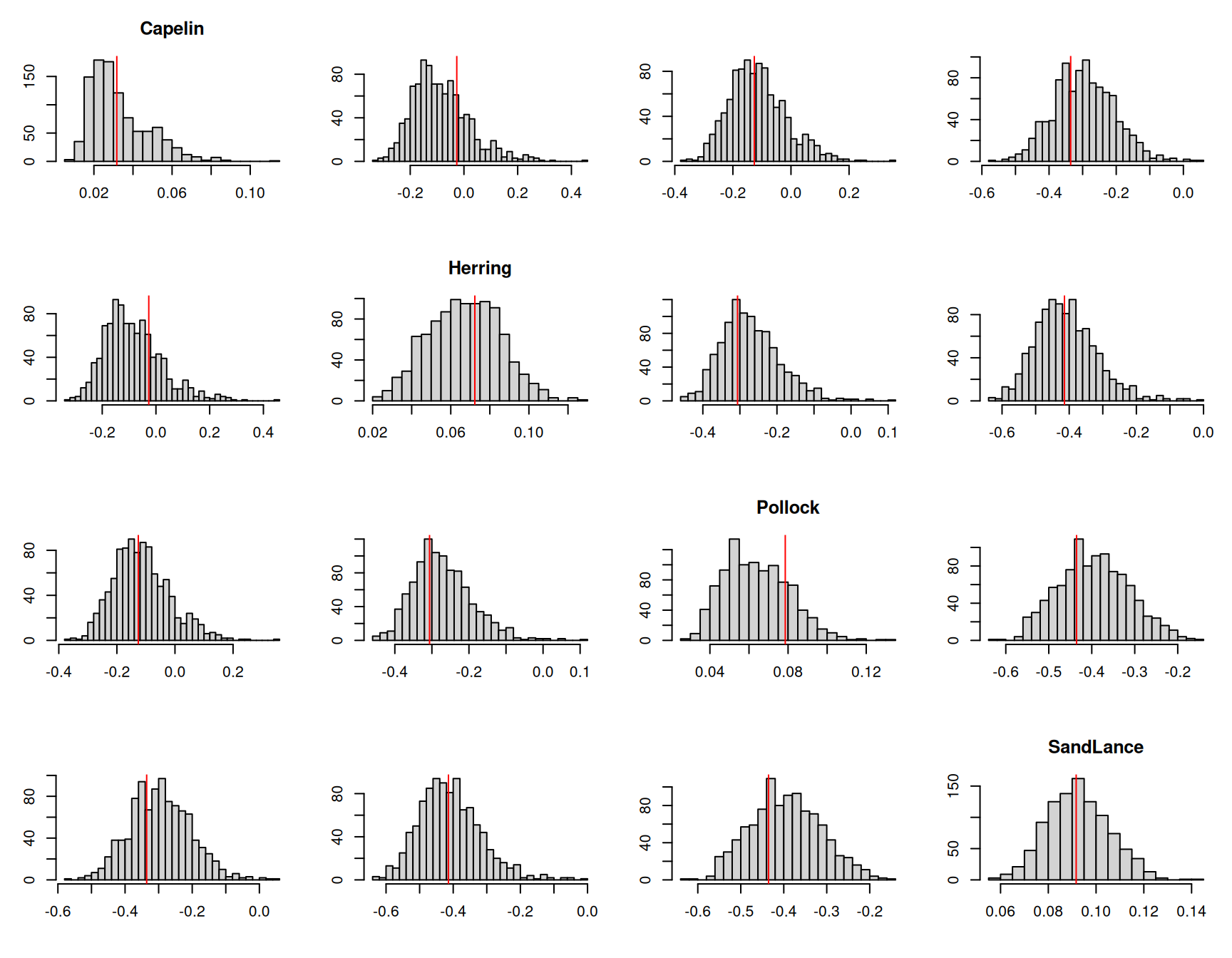
Figure 7.18: The mean proportion of each prey item across samples in a given year were calculated for one thousand posterior predictive simulations from model \(\texttt{m.tuftedc}\). This histograms represent the posterior predictive distributions for the variances of the yearly means (diagonal) or the correlations in yearly means between prey items. The red lines are the values calculated from the data.
We could also consider a similar model for the sample \(\texttt{unit}\) effects:
m.tuftedd<-MCMCglmm(cbind(Capelin, Herring, Pollock, SandLance, Other)~trait-1, data=tufted_puffin, random=~idh(trait):year+year+units, rcov=~idh(trait):units, family="multinomial", longer=20, prior=prior.tufted, pr=TRUE)The magnitude of the units variances show similar patterns to the year variances, with \(\texttt{Other}\) being small and Capelin being large (Table 7.3).
| year | units | |
|---|---|---|
| Capelin | 68.14 [15.38-151.53] | 77.44 [32.96-126.39] |
| Herring | 33.78 [8.89-74.79] | 11.12 [5.05-17.50] |
| Pollock | 12.82 [2.80-26.37] | 4.21 [0.56-7.92] |
| SandLance | 13.35 [3.95-26.65] | 9.91 [5.42-15.20] |
| Other | 1.57 [0.00-5.55] | 3.23 [0.00-6.22] |
Since model \(\texttt{m.tuftedd}\) simplifies the covariance structure of the unit effects compared to previous models, it makes sense to assess the fit of the model by looking at unit-level patterns. To do this, we can simply calculate the proportion of each prey item in a sample and then calculate the variance in these proportions , or the correlation in proportions for pairs of prey items. Figure 7.19 plots the posterior predictive distributions of these quantities and compares them to their observed values.
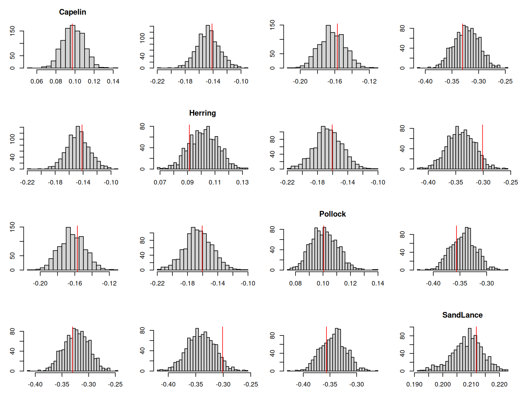
Figure 7.19: The histograms represent the posterior predictive distributions for the variances of the proportion of each prey item in a sample (diagonal) or the correlations in the proportion of prey items in a sample. The red lines are the values calculated from the data.
Generally, the model seems to predict these quantities well, although the correlation between Herring and Sand lance is at the extreme end of that seen in the posterior predictive simulations. This is evidenced in the fully unstructured model where the correlation is estimated to be more positive than all other correlations (Table 7.1).
7.7 Zero-modified Poisson Models
A range of distributions are available for dealing with data where the non-zero counts conform to a Poisson distribution but the frequency of zeros is either too high or too low. The zero-truncated Poisson (ztpoisson) is the most extreme and is for situations where zeros are entirely missing. Three other distributions provide greater flexibility with the zero-inflated Poisson (zipoisson) allowing an excess of zeros and the hurdle Poisson (hupoisson) and the zero-altered Poisson (zapoisson) allowing both excesses and deficits. For these three distributions each data point is associated with two latent variables. The first latent variable is associated with a Poisson distribution and the second latent variable is associated with a Bernoulli distribution. For zero-inflated Poisson models the first latent variable specifies a standard Poisson, and the second latent variable models the probability that a zero belongs to this Poisson (failure) or is from some other process (success). The probability is modelled with logit link. For the hurdle and zero-altered Poissons, the first latent variable specifies a zero-truncated Poisson, and the second latent variable models the probability that an observation is a zero or not. For the hurdle Poisson a zero is a success and the probability is modelled with logit link. For the zero-altered Poisson a non-zero is a success and the complementary log-log link is used. Figure 7.20 provides a graphical representation of these distributions.
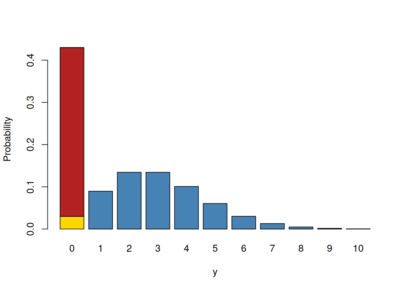
Figure 7.20: Probability mass function for a zero-modified Poisson. The blue and yellow bars combined represent a Poisson distribution with a mean of three. The red bar represents the excess zeros compared to what is expected under the Poisson (in yellow). The blue bars alone represent a zero-truncated distribution. In zero-inflated models, the first latent variable is the mean of the Poisson (blue and yellow bars combined) and the second latent variable models the probability of a zero being in the red category versus the yellow. In hurdle and zero-altered models, the first latent variable is the mean of a zero-truncated Poisson (blue bars) and the second latent variable models the probability of a zero (red and yellow bars combined) versus non-zero (blue bars).
To illustrate these models I’ll use the data bioChemists available in the package \(\texttt{pscl}\). The data were collected on 915 biochemistry graduates and the response variable art is the number of papers published during their PhD.
##   art   fem     mar kid5  phd ment
## 1   0   Men Married    0 2.52    7
## 2   0 Women  Single    0 2.05    6
## 3   0 Women  Single    0 3.75    6
## 4   0   Men Married    1 1.18    3
## 5   0 Women  Single    0 3.75   26
## 6   0 Women Married    2 3.59    2
Approximately, 30% of students do not publish a paper
##
##     FALSE      TRUE
## 0.6994536 0.3005464
which is considerably more than expected from a Poisson distribution with a mean equal to the mean number of papers published (1.69).
## [1] 0.1839859If we compare the observed frequencies of the number of papers published with a standard Poisson, we can see than not only is there an excess of zero’s but also an excess of students publishing four or more papers (Figure 7.21).
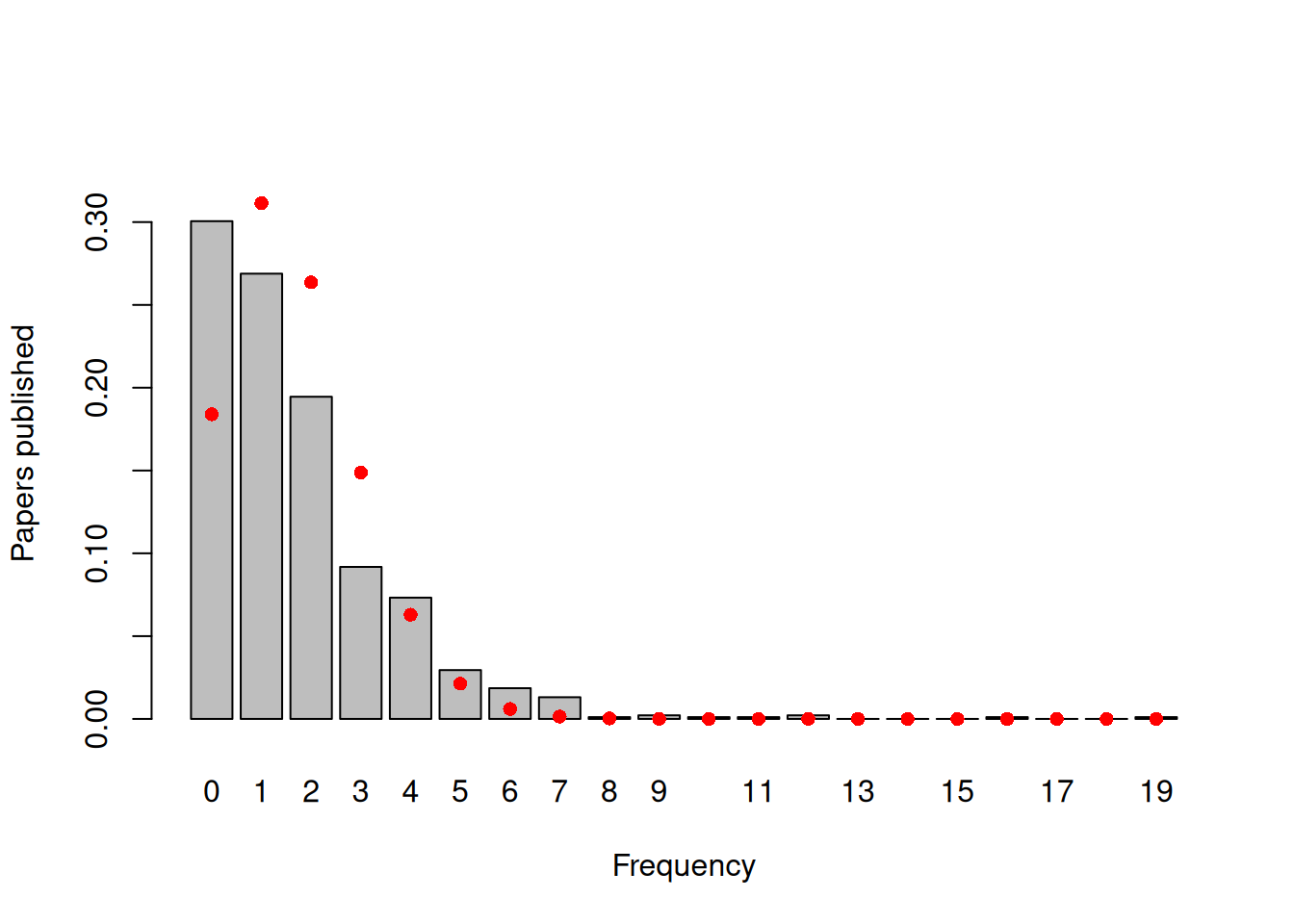
Figure 7.21: Number of papers published by biochemistry graduate students during their PhD. The red dots are the probabilities calculated from a Poisson with a mean of 1.69.
While the excess of zeros may suggest that the distribution is zero-inflated, general overdispersion will also create an excess of zeros. If we focus only on the non-zero counts and compare their distribution to what we would expect under a zero-truncated Poisson, an excess of small values and very large values is evident - the non-zero data are overdispersed with respect to the zero-truncated Poisson (Figure 7.22). As is often the case, it’s unclear whether the large number of zero’s in the data are due to zero-inflation or overdispersion more generally.
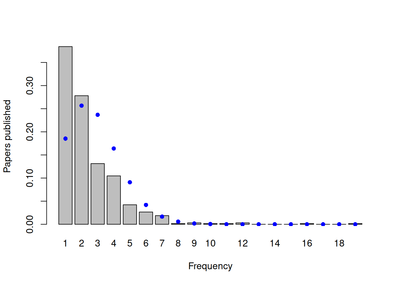
Figure 7.22: Number of papers published by biochemistry graduate students during their PhD, excluding those students that published no papers. The blue dots are the probabilities calculated from a zero-truncated Poisson with a mean of 2.42.
As with standard Poisson models, by allowing observation-level (\(\texttt{unit}\)) effects, MCMCglmm fits an overdispersed (zero-truncated) Poisson when fitting zero-modified Poisson distributions (Section 3.4.2). Consequently, any zero-modification is with respect to the overdispersed distribution. As in Bernoulli models, \(\texttt{unit}\) effects are fitted in the zero-modification model, but their variance is not identifiable and so should usually be fixed in the prior (Section 3.6.3). Similarly, any covariation between the Poisson model and the zero-modification model at the level of an observation is not identifiable, since non-zero Poisson counts are absent for all observations that have zero counts, obviously. Consequently, the residual covariance matrix for the pair of latent variables is usually constrained to have the form:
\[ V_{\texttt{units}} =\left[ \begin{array}{cc} \sigma^2_{y}&0\\ 0&1\\ \end{array} \right] \]
where \(\sigma^2_{y}\) is the units variance for the (zero-truncated) Poisson. This can be achieved by using an \(\texttt{idh}\) structure and fixing the second variance to one by specifying \(\texttt{fix}\) in the prior.
7.7.1 Zero-inflated Poisson
To the biochemsirty student data, we can fit a zero-inflated model where we specify constant odds for a zero belonging to the inflation process rather than the Poisson process, but the mean of the Poisson may depend on a suite of predictors such as the categorical predictors sex (\(\texttt{fem}\)) and marital status (\(\texttt{Married}\)) and continuous predictors such as the number of children aged 5 or younger (\(\texttt{kid5}\)) prestige of the department (\(\texttt{phd}\)) and how many papers the student’s mentor published over the same period (\(\texttt{ment}\)).
prior.zip=list(R=list(V=diag(2), nu=0.002, fix=2))
m.zip<-MCMCglmm(art~trait-1+at.level(trait,1):(fem + mar + kid5 + phd +ment), rcov=~idh(trait):units, data=bioChemists, prior=prior.zip, family="zipoisson", longer=10)
Let’s look at the model summary:
##
##  Iterations = 30001:129901
##  Thinning interval  = 100
##  Sample size  = 1000
##
##  DIC: 3021.529
##
##  R-structure:  ~idh(trait):units
##
##                   post.mean l-95% CI u-95% CI eff.samp
## traitart.units       0.3972   0.2951   0.4904    353.8
## traitzi_art.units    1.0000   1.0000   1.0000      0.0
##
##  Location effects: art ~ trait - 1 + at.level(trait, 1):(fem + mar + kid5 + phd + ment)
##
##                                post.mean   l-95% CI   u-95% CI eff.samp  pMCMC
## traitart                       -0.169215  -0.443890   0.117923   649.77  0.238
## traitzi_art                    -7.719087 -14.715896  -2.610300     2.53 <0.001
## at.level(trait, 1):femMen       0.204749   0.064065   0.342074  1171.70  0.004
## at.level(trait, 1):marMarried   0.151521  -0.006506   0.328658  1000.00  0.074
## at.level(trait, 1):kid5        -0.177760  -0.285810  -0.077662  1000.00  0.002
## at.level(trait, 1):phd          0.027820  -0.054340   0.090490  1122.33  0.458
## at.level(trait, 1):ment         0.027788   0.021779   0.033844  1000.00 <0.001
##
## traitart
## traitzi_art                   ***
## at.level(trait, 1):femMen     **
## at.level(trait, 1):marMarried .
## at.level(trait, 1):kid5       **
## at.level(trait, 1):phd
## at.level(trait, 1):ment       ***
## ---
## Signif. codes:  0 '***' 0.001 '**' 0.01 '*' 0.05 '.' 0.1 ' ' 1
The first ‘trait’ has the same name as the response (\(\texttt{art}\) in this example) and is the latent variable for the Poisson process. The second ‘trait’ is the latent variable for the zero-inflation and has the same name as the response prefixed by \(\texttt{zi_}\) (\(\texttt{zi_art}\)). We can see that there is good evidence for overdispersion: the \(\texttt{units}\) variance for the Poisson process (\(\texttt{traitart.units}\)) is far from zero and several of the covariates seem to impact the Poisson mean. However, note that the log odds of a zero belonging to the zero-inflation process is extremely small (-7.72) - essentially a probability of zero - and the mixing is very poor for this parameter which has a very low effective sample size. We can see this visually by looking at the MCMC traces from the model (Figure 7.23).
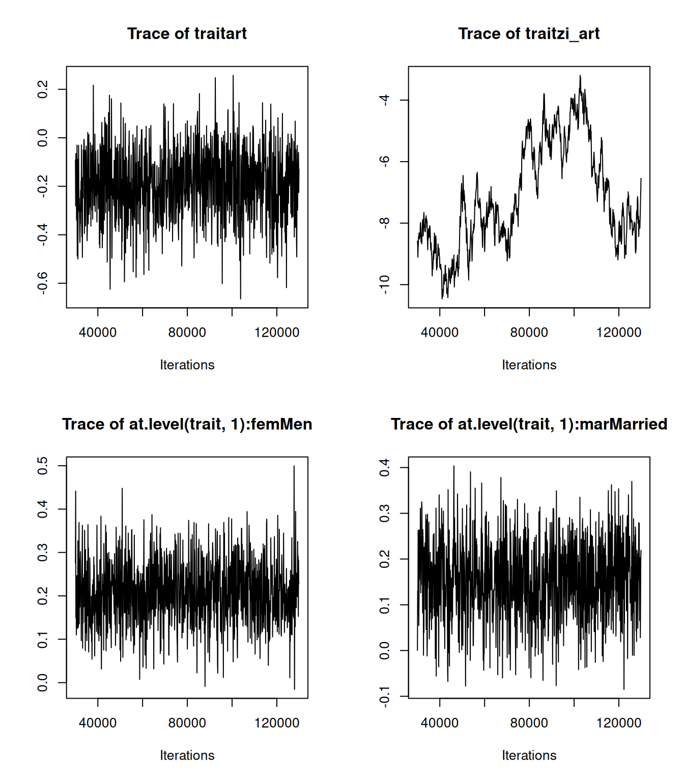
Figure 7.23: MCMC traces for the first four fixed effects from the zero-inflated Poisson model m.zip in which trait 1 (\(\texttt{art}\)) is the Poisson process and trait 2 (\(\texttt{zi.art}\)) is the zero-inflation.
The reason that the model mixes so poorly for the zero-inflation parameter is that there is essentially no zero-inflation. We have complete separation where the likelihood is favouring estimates of the probability that are close to zero and therefore minus infinity on the logit scale (Section 3.9). Before worrying about zero-inflation I usually fit a standard (over-dispersed) Poisson:
prior.odp=list(R=list(V=diag(1), nu=0.002))
m.odp<-MCMCglmm(art~fem + mar + kid5 + phd + ment, data=bioChemists, prior=prior.odp, family="poisson")
and then use posterior predictive checks to see how many zero’s you would expect under this simpler model:
# simulate from model
ysim<-simulate(m.odp, nsim=1000)

# count the number of zeros for each simulated data set
nzsim<-colSums(ysim==0)

# plot posterior predictive distribution with observed value
hist(nzsim, main="", xlab="Number of zeros")
abline(v=sum(bioChemists$art==0), col="red", lwd=2)
Figure 7.24: Posterior predictive distribution from an (overdispersed) Poisson model fitted to the number of biochemistry students (out of 915) that publish no papers during their PhD. The red line is the observed number.
The simpler model seems to be entirely consistent with the number of zeros (Figure 7.24) suggesting that a zero-inflated model may not be required.
7.7.2 Hurdle Poisson models
In hurdle and zero-altered models, it is the probability of a zero versus non-zero that is modelled, rather than the probability a zero belongs to the zero-inflation process (Figure 7.20). Consequently, complete separation only occurs when no zeros are observed and the probability tends to zero. The equivalent model to \(\texttt{m.zip}\) but using a hurdle distribution therefore behaves better
m.hup<-MCMCglmm(art~trait-1+at.level(trait,1):(fem + mar + kid5 + phd +ment), rcov=~idh(trait):units, data=bioChemists, prior=prior.zip, family="hupoisson", longer=10)
summary(m.hup)
##
## Iterations = 30001:129901
## Thinning interval = 100
## Sample size = 1000
##
## DIC: 3106.443
##
## R-structure: ~idh(trait):units
##
## post.mean l-95% CI u-95% CI eff.samp
## traitart.units 0.3555 0.2485 0.4669 630.4
## traithu_art.units 1.0000 1.0000 1.0000 0.0
##
## Location effects: art ~ trait - 1 + at.level(trait, 1):(fem + mar + kid5 + phd + ment)
##
## post.mean l-95% CI u-95% CI eff.samp pMCMC
## traitart 0.14783 -0.15160 0.46039 763.7 0.384
## traithu_art -1.01029 -1.16686 -0.81848 1000.0 <0.001 ***
## at.level(trait, 1):femMen 0.20113 0.02404 0.36258 1000.0 0.008 **
## at.level(trait, 1):marMarried 0.08908 -0.08282 0.29976 1000.0 0.346
## at.level(trait, 1):kid5 -0.13458 -0.27209 -0.01632 1000.0 0.038 *
## at.level(trait, 1):phd 0.01341 -0.06609 0.09980 744.7 0.760
## at.level(trait, 1):ment 0.01956 0.01239 0.02649 1000.0 <0.001 ***
## ---
## Signif. codes: 0 '***' 0.001 '**' 0.01 '*' 0.05 '.' 0.1 ' ' 1Compared to the zero-inflated traces plotted in Figure 7.23 the equivalent parameters in the hurdle model show better mixing (Figure 7.25).
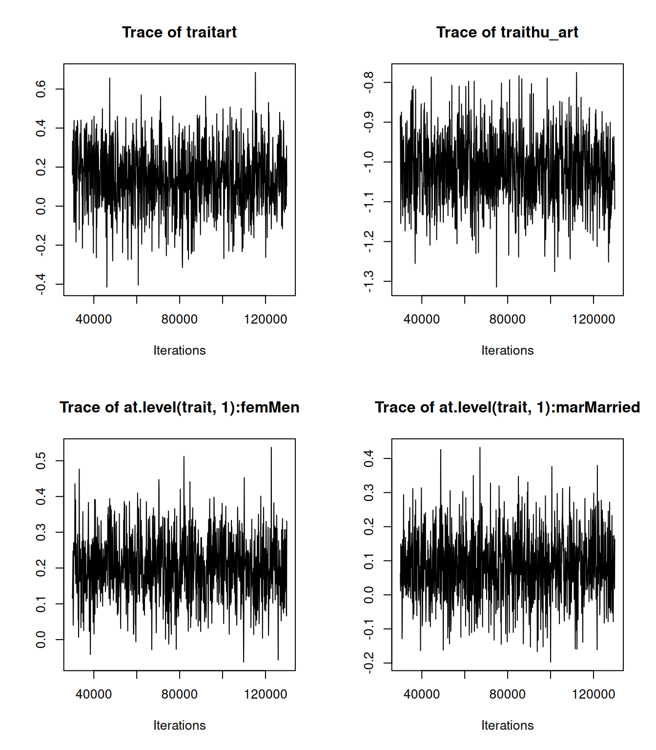
Figure 7.25: MCMC traces for the first four fixed effects from the hurdle Poisson model m.hup in which trait 1 (\(\texttt{art}\)) is the Poisson process and trait 2 (\(\texttt{zi.art}\)) is the probability of being zero.
However, the interpretation of the hurdle model is slightly different than the zero-inflated model. In the hurdle model, fitting just an intercept for the zero-modification process implies that the proportion of zeros observed across different combinations of fixed effects is constant. Our 95% credible intervals for this proportion is (See section 3.6.2):
##          lower     upper
## var1 0.2657294 0.3283723
## attr(,"Probability")
## [1] 0.95
While this is consistent with the overall frequency of zeros in the data set it is unclear whether it is consistent with the observed frequency of zeros across different groups of students. For example, the frequency of zero’s is perhaps lower in men than women and increases with the number of children under 5 (there is only one observation for a women with 3 children under 5).
##               0         1         2         3
## Men   0.2441860 0.2877698 0.3170732 0.4666667
## Women 0.3255132 0.3214286 0.4347826 0.0000000
In standard and zero-inflated Poisson models, these frequencies would be expected to change depending on how the predictors affect the mean number of papers (including zeros). For example, when we fitted the standard Poisson model to these data the predicted frequency of zeros is:
ysim<-simulate(m.odp, nsim=1000)==0
ysim<-apply(ysim, 1, sum)/1000

tapply(ysim, list(bioChemists$fem, bioChemists$kid5), mean)
## 0 1 2 3
## Men 0.2475814 0.2734820 0.3222439 0.4166
## Women 0.3200704 0.3479821 0.3827826 0.4160which largely recapitulates what is seen in the data. We can relax the assumption of a fixed proportion of zeros by fitting the same predictors for the zero-modified process
m.hup2<-MCMCglmm(art~trait-1+trait:(fem+mar+kid5+phd+ment), rcov=~idh(trait):units, data=bioChemists, prior=prior.zip, family="hupoisson", longer=10)
summary(m.hup2)
##
## Iterations = 30001:129901
## Thinning interval = 100
## Sample size = 1000
##
## DIC: 3047.131
##
## R-structure: ~idh(trait):units
##
## post.mean l-95% CI u-95% CI eff.samp
## traitart.units 0.3529 0.2429 0.4605 584.9
## traithu_art.units 1.0000 1.0000 1.0000 0.0
##
## Location effects: art ~ trait - 1 + trait:(fem + mar + kid5 + phd + ment)
##
## post.mean l-95% CI u-95% CI eff.samp pMCMC
## traitart 0.336746 -0.003901 0.660538 898.1 0.050 .
## traithu_art -0.286291 -0.937922 0.463449 1000.0 0.410
## traitart:femWomen -0.197487 -0.357091 0.004876 1000.0 0.042 *
## traithu_art:femWomen 0.294816 -0.081355 0.623314 1097.5 0.100
## traitart:marMarried 0.088297 -0.119298 0.285623 1000.0 0.398
## traithu_art:marMarried -0.386799 -0.826199 -0.002998 1000.0 0.056 .
## traitart:kid5 -0.130792 -0.259294 -0.003182 1000.0 0.048 *
## traithu_art:kid5 0.331153 0.060392 0.591070 801.0 0.016 *
## traitart:phd 0.016407 -0.057650 0.100150 1000.0 0.716
## traithu_art:phd -0.031913 -0.217134 0.162858 1000.0 0.756
## traitart:ment 0.019494 0.012362 0.026042 1000.0 <0.001 ***
## traithu_art:ment -0.092044 -0.119956 -0.061384 578.3 <0.001 ***
## ---
## Signif. codes: 0 '***' 0.001 '**' 0.01 '*' 0.05 '.' 0.1 ' ' 1However, the fully parameterised model involves almost doubling the number of location parameters. This highlights one of the disadvantages of hurdle models. If zeros do arise through the same process that generate the non-zero counts (either with zero-inflation or not) then the proportion of zero’s observed across a set of explanatory variables will vary if those predictors affect the expectation of the Poisson. It may then be necessary to fit an equally complicated model for both processes even though no additional parameter would be required if the model was fitted as a standard Poisson and a single intercept parameter may suffice in a zero-inflated model if there were excess zeros.
7.7.3 Zero-altered Poisson Models
Zero-altered Poisson (ZAP) models are identical to Poisson hurdle models except the second latent variable models the probability of a non-zero (rather than a zero) and the complementary log-log link is used40. The motivation behind this is that the standard Poisson can then become a special case of the zero-altered Poisson. With complementary log-log link, the probability of a zero is equal to \(exp(-exp(l_2))\), where \(l_2\) is the second latent variable. The probability of obtaining a zero from a Poisson distribution with mean \(\lambda\) is \(exp(-\lambda)\). Consequently, in a Poisson GLM with log-link, the probability of a zero is \(exp(-exp(l_1))\), where \(l_1\) is the first latent variable. Applying the constraint that \(l_1=l_2\) across all observations, the zero-altered Poisson model is equivalent to the standard Poisson. In MCMCglmm, \(l_1\) and \(l_2\) cannot be constrained to be equal because they must at least differ in their residual, since each ‘trait’ must have a unique residual. Nevertheless, the residuals can be forced to have the same residual (\(\texttt{unit}\)) variance, although all of the information comes from the Poisson part.
m.zap1<-MCMCglmm(art~fem+mar+kid5+phd+ment, rcov=~trait:units, data=bioChemists, family="zapoisson", prior=prior.odp, longer=10)
summary(m.zap1)
##
## Iterations = 30001:129901
## Thinning interval = 100
## Sample size = 1000
##
## DIC: 3033.201
##
## R-structure: ~trait:units
##
## post.mean l-95% CI u-95% CI eff.samp
## trait:units 0.4245 0.3346 0.5382 653.2
##
## Location effects: art ~ fem + mar + kid5 + phd + ment
##
## post.mean l-95% CI u-95% CI eff.samp pMCMC
## (Intercept) 0.093893 -0.195988 0.346553 1000.0 0.496
## femWomen -0.201294 -0.333646 -0.054387 1170.3 0.004 **
## marMarried 0.150736 0.002764 0.308497 826.2 0.056 .
## kid5 -0.172630 -0.273023 -0.071454 830.2 0.002 **
## phd 0.030223 -0.043338 0.097853 947.7 0.392
## ment 0.027010 0.021281 0.033506 1000.0 <0.001 ***
## ---
## Signif. codes: 0 '***' 0.001 '**' 0.01 '*' 0.05 '.' 0.1 ' ' 1If we plot the coefficients and \(\texttt{units}\) variance for this model and compare it to the standard (overdispersed) Poisson we see that the posteriors are in close agreement, for all but the intercept (Figure 7.26). The difference in intercept presumably arises because of the separate \(\txttt{unit}\) effect for the two processes.
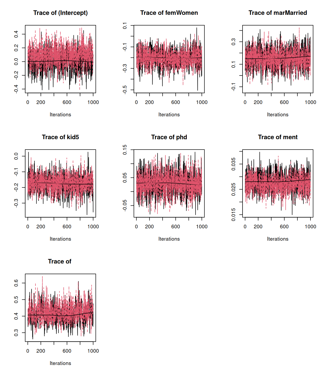
Figure 7.26: In red is are the MCMC traces for the fixed effects and $ exttt{units}$ variance from the zero-inflated Poisson model m.zap1 in which trait 1 (\(\texttt{art}\)) is the Poisson process and trait 2 (\(\texttt{zi.art}\)) is the probability of being zero. The MCMC traces in black are from the equivalent overdispersed Poisson model, m.odp.
Consequently, we can test for zero-modification by setting up the contrasts so that the zero-altered regression coefficients are expressed as differences from the Poisson regression coefficients. When this difference is zero the variable causes no zero-modification, when it is negative it causes zero-inflation and when it is positive it causes zero-deflation:
m.zap2<-MCMCglmm(art~trait*(fem +mar + kid5 + phd + ment), rcov=~trait:units, data=bioChemists, prior=prior.odp, family="zapoisson", longer=10)
summary(m.zap2)
##
## Iterations = 30001:129901
## Thinning interval = 100
## Sample size = 1000
##
## DIC: 3039.872
##
## R-structure: ~trait:units
##
## post.mean l-95% CI u-95% CI eff.samp
## trait:units 0.3636 0.2551 0.4747 438.3
##
## Location effects: art ~ trait * (fem + mar + kid5 + phd + ment)
##
## post.mean l-95% CI u-95% CI eff.samp pMCMC
## (Intercept) 0.332009 -0.028021 0.654377 869.3 0.070 .
## traitza_art -0.540884 -1.118145 -0.056006 452.2 0.058 .
## femWomen -0.201123 -0.371123 -0.030718 1000.0 0.032 *
## marMarried 0.091881 -0.092843 0.279585 1000.0 0.366
## kid5 -0.131154 -0.250644 -0.006522 898.9 0.032 *
## phd 0.016314 -0.065377 0.101470 1000.0 0.696
## ment 0.019394 0.012961 0.026964 1000.0 <0.001 ***
## traitza_art:femWomen 0.038288 -0.254231 0.303005 1000.0 0.768
## traitza_art:marMarried 0.146334 -0.189678 0.430403 1000.0 0.334
## traitza_art:kid5 -0.074948 -0.247521 0.116607 969.6 0.446
## traitza_art:phd 0.010214 -0.124226 0.144946 1000.0 0.894
## traitza_art:ment 0.028568 0.013046 0.045079 830.6 0.002 **
## ---
## Signif. codes: 0 '***' 0.001 '**' 0.01 '*' 0.05 '.' 0.1 ' ' 1The credible intervals on the interaction coefficients (including traitza_art) are large and so drawing firm conclusions is hard, although there does seem that the more papers a mentor produces, the more zero-deflation (or conversely the less papers a mentor produces, the more zero-inflation).
If the model has >2 responses and you want to regress response \(\texttt{i}\) effects on the remainder (i.e. a multiple regression), the coefficients can be obtained as
solve(V[-i,-i], V[i,-i])where \(\texttt{V}\) is the (co)variance matrix of effects.↩︎We could also have parameterised the model directly as a regression using \(\texttt{ante1(trait):id}\) \(\texttt{ante1(trait):units}\) - see Section 6.5.↩︎
If we had an additional covariate, let’s say \(\texttt{rain}\), we can also obtain the \(\texttt{units}\) variance had we fitted both \(\texttt{rain}\) and \(\texttt{ice}\). Define \({\bf c}\) as the \(2\times 1\) vector of residual covariances between road accidents and the weather variables and \({\bf V}\) as the \(2\times 2\) residual covariance matrix for the weather variables. Then \(\sigma^2_\texttt{traity|weather.unit} = \sigma^2_\texttt{traity.unit}-{\bf c}^{\top}{\bf V}^{-1}{\bf c}\).↩︎
For a \(2\times 2\) covariance matrix, positive-definitness requires both variances to be positive and the correlation to lie between -1 and 1. For covariance matrices of larger dimension, the conditions for positive-definitness are more complicated. Perhaps the simplest definition is that all eigenvalues are positive. The function \(\texttt{posterior.evals}\) returns the posterior distribution of the \(k\) eigenvalues given the posterior samples of a \(k\) dimensional covariance matrix (obtained for the appropriate \(k^2\) columns of the \(\texttt{VCV}\) element of the \(\texttt{MCMCglmm}\) model object.)↩︎
\(\texttt{at.level}\) takes the name of categorical variable together with a vector of specified levels. It creates an \(n\times k\) incidence matrix where \(n\) is the length of the categorical variable and \(k\) the number of specified levels. The matrix element \(ij\) has a one if the categorical variable for observation \(i\)is of level \(j\), and zero otherwise. When \(\texttt{at.level}\) is used in a model formula, and interacted with other terms, it restricts those terms to only having effects when the observations are associated with the \(k\) specified levels. For example, imagine a categorical variable \(\texttt{fac}\) with three levels \(\texttt{a}\), \(\texttt{b}\), and \(\texttt{c}\) and a continuous variable \(\texttt{x}\). \(\texttt{at.level(fac, c("a", "c")):x}\) would fit two effects - an effect of \(x\) when \(\texttt{fac}=\texttt{a}\) and an effect of \(x\) when \(\texttt{fac}=\texttt{c}\). \(\texttt{at.set}\) is similar although it creates an \(n\times 1\) incidence matrix where element \(i\) is one if the categorical variable for observation \(i\) is any of the specified levels. The term \(\texttt{at.set(fac, c("a", "c")):x}\) would then fit one effect - the effect of \(x\) when \(\texttt{fac}\) is equal to \(\texttt{a}\) or \(\texttt{c}\).↩︎
For more complicated models a (co)variance matrix may be estimated for a particular random component rather than just a single variance as here. In such cases,
Vis a matrix. The value at which (part of) the (co)variance matrix is fixed at is determined byV. Any elements of the covariance matrix in rows and/or columns equal to or greater thanfixare fixed. In the case of a single variancefix=1simply fixes the variance (element 1,1 of the (co)variance matrix) at whatever is specified inV(one in this example).↩︎Obtaining this expression is involved. We can express the expected value of \(y\) given \(l\) is less than, or greater than, some value \(c\) using the law of total expectation
\[E[y | l>c] = E[E[y|l] | l>c]\]
and
\[E[y | l<c] = E[E[y|l] | l<c]\]
\(E[y|l]\) is the mean of a conditional normal which has a well known form: \(\mu_y+\frac{\sigma_{y,l}}{\sigma^2_{l}}(l-\mu_l)\). The expectation of this when \(l>c\) is then \(\mu_y+\frac{\sigma_{y,l}}{\sigma^2_{l}}(E[l|l>c]-\mu_l)\). \(E[l|l>c]\) can be obtained using the inverse Mills ratio:
\[E[l|l>c] = \mu_l + \sigma_{l}\frac{f_N(\alpha)}{(1 - F_N(\alpha))}\]
and when \(l<c\) we have
\[E[l|l<c] = \mu_l - \sigma_{l}\frac{f_N(\alpha)}{F_N(\alpha)}\]
where \(f_N\) and \(F_N\) are the density and cumulative density functions for the unit normal, and \(\alpha = \mu_l/\sigma_{l}\). Code for obtaining \(E[y | l>c]\) and \(E[y | l>c]\) can be foundhere
condE <- function(mu, V, c=0, greater=TRUE) { # A bivariate normal with mean vector mu and covariance matrix V is assumed. # condE give expectation of 1st variable given 2nd variable is > c (greater=TRUE) or < c (greater=FALSE) if(nrow(V)!=ncol(V) | nrow(V)!=2){ stop("V should be a 2x2 matrix") } if(length(mu)!=2){ stop("mu should be length 2") } alpha <- (c - mu[2]) /sqrt(V[2,2]) if(greater){ lambda <- dnorm(alpha)/(1 - pnorm(alpha)) # inverse Mills ratio expectation<- mu[2] + sqrt(V[2,2])*lambda }else{ lambda <- dnorm(alpha)/pnorm(alpha) expectation<- mu[2] - sqrt(V[2,2])*lambda } # Expectation that E[l|l>0] or E[l|l<0] expectation<-mu[1]+(expectation-mu[2])*V[1,2]/V[2,2] # Expectation of x given l|l>0. # The whole thing simplifies to # mu[1] \pm lambda*V[1,2]/sqrt(V[2,2]) # but easier to see the logic without the simplification return(expectation) }I should really have an na.option in the call to \(\texttt{MCMCglmm}\) that simply ignores missing values in the wide-format.↩︎
Obtaining comparable regression coefficients between the single and multi-response models is fairly involved. The reason for this is that the standard single-response probit model assumes a \(\texttt{units}\) variance of one after conditioning on the predictors, yet the multiple-response model assumes a \(\texttt{units}\) variance of one before conditioning on the predictors. Nevertheless, we can easily move between the two parameterisations. As detailed at the start of this Chapter and in the footnote[^schur], the $ variance for death after conditioning on the \(\texttt{id}\) effects for \(log(\texttt{bili})\) is \(V_{2|1}=V_{2,2}-V_{1,2}^2/V_{1,1}\) where \({\bf V}\) is the covariance matrix. As covered in Section 3.6.3 and in footnote[^3.5] we can then rescale the regression coefficient from the multi-response model by \(\sqrt{2/(1+V_{2|1})}\) to obtain the value we get if we could have set \(V_{2|1}=1\) as in the single-response model.↩︎
An identity matrix has ones along the diagonal and zero’s on the off-diagonals. A unit matrix is a matrix of all ones.↩︎
It is not immediately obvious what this is doing. The model formula specifies five parameters across the four traits. The term \(\texttt{trait}\) defines four effects, one effect for each trait since the intercept is suppressed for formula inside variance functions. The term
at.set(trait, 1:4sets up a single binary indicator variable with a one when the trait level is 1, 2, 3, or 4. Since this is all the four traits, this is just setting up a column of ones. The associated parameter is common to all traits and this will be our \(\texttt{Other}\) effect. If we interact the variance structure with year we end up with a set of five year effects for year \(j\) with design matrix:\[{\bf Z}_j=\left[\begin{array}{ccccc} 1&0&0&0&1\\ 0&1&0&0&1\\ 0&0&1&0&1\\ 0&0&0&1&1\\ \end{array}\right] \]
The \(\texttt{idv}\) variance structure assumes the five effects are uncorrelated with a common variance, such that \(\sigma^2_u{\bf Z}_j{\bf Z}^{\top}_j = \sigma^2_u({\bf I}+{\bf J})\): the specification is equivalent to just fitting four year effects with the desired covariance structure.↩︎
I can now find no reference of this model being referred to as a zero-altered model, but for back compatibility it will have to remain as
zapoisson.↩︎