Multivariate Generalised Linear Mixed Models

Markov chain Monte Carlo Sampler for Multivariate Generalised Linear Mixed Models with special emphasis on correlated random effects arising from pedigrees and phylogenies (Hadfield 2010). Please read the course notes: vignette("CourseNotes", "MCMCglmm") or the overview vignette("Overview", "MCMCglmm")

Usage

MCMCglmm(fixed, random=NULL, rcov=~units, family="gaussian", mev=NULL, 
    data,start=NULL, prior=NULL, tune=NULL, pedigree=NULL, nodes="ALL",
    scale=TRUE, nitt=13000, thin=10, burnin=3000, pr=FALSE,
    pl=FALSE, verbose=TRUE, DIC=TRUE, singular.ok=FALSE, saveX=TRUE,
    saveZ=TRUE, saveXL=TRUE, slice=FALSE, ginverse=NULL, trunc=FALSE, 
    theta_scale=NULL, saveWS=TRUE, aggregate=NULL, longer=1)

Arguments

fixed: formula for the fixed effects, multiple responses are passed as a matrix using cbind
random: formula for the random effects. Multiple random terms can be passed using the + operator, and in the most general case each random term has the form variance.function(formula):linking.function(random.terms). Currently, the only variance.functions available are idv, idh, us, cor[] and ante[]. idv fits a constant variance across all components in formula. Both idh and us fit different variances across each component in formula, but us will also fit the covariances. corg fixes the variances along the diagonal to one and corgh fixes the variances along the diagonal to those specified in the prior. cors allows correlation submatrices. ante[] fits ante-dependence structures of different order (e.g ante1, ante2), and the number can be prefixed by a c to hold all regression coefficients of the same order equal. The number can also be suffixed by a v to hold all innovation variances equal (e.g antec2v has 3 parameters). The formula can contain both factors and numeric terms (i.e. random regression) although it should be noted that the intercept term is suppressed. The (co)variances are the (co)variances of the random.terms effects. Currently, the only linking.functions available are mm and str. mm fits a multimembership model where multiple random terms are separated by the + operator. str allows covariances to exist between multiple random terms that are also separated by the + operator. In both cases the levels of all multiple random terms have to be the same. For simpler models the variance.function(formula) and linking.function(random.terms) can be omitted and the model syntax has the simpler form ~random1+random2+.... There are two reserved variables: units which index rows of the response variable and trait which index columns of the response variable
rcov: formula for residual covariance structure. This has to be set up so that each data point is associated with a unique residual. For example a multi-response model might have the R-structure defined by ~us(trait):units
family: optional character vector of trait distributions. Currently, "gaussian", "poisson", "categorical", "multinomial", "ordinal", "threshold", "exponential", "geometric", "cengaussian", "cenpoisson", "cenexponential", "zipoisson", "zapoisson", "ztpoisson", "hupoisson", "zibinomial", "threshold", "nzbinom" , "ncst", "msst" , "hubinomial", "ztmb" and "ztmultinomial" are supported, where the prefix "cen" means censored, the prefix "zi" means zero inflated, the prefix "za" means zero altered, the prefix "zt" means zero truncated and the prefix "hu" means hurdle. If NULL, data needs to contain a family column.
mev: optional vector of measurement error variances for each data point for random effect meta-analysis.
data: data.frame
start: optional list having 5 possible elements: R (R-structure) G (G-structure) and Liab (latent variables or liabilities) should contain the starting values where G itself is also a list with as many elements as random effect components. The element QUASI should be logical: if TRUE starting latent variables are obtained heuristically, if FALSE then they are sampled from a Z-distribution. The element r should be be between -1 and 1 and determines the correlation between the starting latent variables and the ordered latent variables (ordered by the response variable): the default is 0.8.
prior: optional list of prior specifications having 4 possible elements: R (R-structure) G (G-structure), B (fixed effects) and S (theta_scale parameter). B and S are lists containing the expected value (mu) and a (co)variance matrix (V) representing the strength of belief: the defaults are B$mu=S$mu=0 and B$V=S$V=I*1e+10, where where I is an identity matrix of appropriate dimension. The priors for the variance structures (R and G) are lists with the expected (co)variances (V) and degree of belief parameter (nu) for the inverse-Wishart (note this parameterisation is non-standard - see rIW), and also the mean vector (alpha.mu) and covariance matrix (alpha.V) for the redundant working parameters. The defaults are nu=0, V=1, alpha.mu=0, and alpha.V=0. When alpha.V is non-zero, parameter expanded algorithms are used.
tune: optional list with elements mh_V and/or mh_weights mh_V should be a list with as many elements as there are R-structure terms with each element being the (co)variance matrix defining the proposal distribution for the associated latent variables. If NULL an adaptive algorithm is used which ceases to adapt once the burn-in phase has finished. mh_weights should be equal to the number of latent variables and acts as a scaling factor for the proposal standard deviations.
pedigree: ordered pedigree with 3 columns id, dam and sire or a phylo object. This argument is retained for back compatibility - see ginverse argument for a more general formulation.
nodes: pedigree/phylogeny nodes to be estimated. The default, "ALL" estimates effects for all individuals in a pedigree or nodes in a phylogeny (including ancestral nodes). For phylogenies "TIPS" estimates effects for the tips only, and for pedigrees a vector of ids can be passed to nodes specifying the subset of individuals for which animal effects are estimated. Note that all analyses are equivalent if omitted nodes have missing data but by absorbing these nodes the chain max mix better. However, the algorithm may be less numerically stable and may iterate slower, especially for large phylogenies.
scale: logical: should the phylogeny (needs to be ultrametric) be scaled to unit length (distance from root to tip)?
nitt: number of MCMC iterations
thin: thinning interval
burnin: burnin
pr: logical: should the posterior distribution of random effects be saved?
pl: logical: should the posterior distribution of latent variables be saved?
verbose: logical: if TRUE MH diagnostics are printed to screen
DIC: logical: if TRUE deviance and deviance information criterion are calculated
singular.ok: logical: if FALSE linear dependencies in the fixed effects are removed. if TRUE they are left in an estimated, although all information comes form the prior
saveX: logical: save fixed effect design matrix
saveZ: logical: save random effect design matrix
saveXL: logical: save structural parameter design matrix
slice: logical: should slice sampling be used? Only applicable for binary traits with independent residuals
ginverse: a list of sparse inverse matrices (${\bf A^{-1}}$) that are proportional to the covariance structure of the random effects. The names of the matrices should correspond to columns in data that are associated with the random term. All levels of the random term should appear as rownames for the matrices.
trunc: logical: should latent variables in binary models be truncated to prevent under/overflow (+/-20 for categorical/multinomial models and +/-7 for threshold/probit models)?
theta_scale: optional list of 4 possible elements specifying a set of location effects (fixed or random) that are to be scaled by the parameter theta_scale for the subset of observations which have level level in factor factor: factor, level, fixed (position of fixed terms to be scaled) and random (position of random effect components).
saveWS: logical: save design matrix for scaled effects.
aggregate: character: names of long-format variables to be formed from wide-format variables in multi-trait models. Wide-format variables should have the long-format variable name followed by an underscore and then the trait name. For example, a wide-format data frame might have variable names y1, y2, x_y1, x_y2. If a multi-trait model is fitted for y1 and y2 then aggregate="x" generates the new variable x=c(x_y1, x_y2).
longer: positive integer that multiples nitt, thin and burnin

Value

Sol: Posterior Distribution of MME solutions, including fixed effects
VCV: Posterior Distribution of (co)variance matrices
CP: Posterior Distribution of cut-points from an ordinal model
Liab: Posterior Distribution of latent variables
Fixed: list: fixed formula and number of fixed effects
Random: list: random formula, dimensions of each covariance matrix, number of levels per covariance matrix, and term in random formula to which each covariance belongs
Residual: list: residual formula, dimensions of each covariance matrix, number of levels per covariance matrix, and term in residual formula to which each covariance belongs
Deviance: deviance -2*log(p(y|...))
DIC: deviance information criterion
X: sparse fixed effect design matrix
Z: sparse random effect design matrix
XL: sparse structural parameter design matrix
error.term: residual term for each datum
family: distribution of each datum
Tune: (co)variance matrix of the proposal distribution for the latent variables
meta: logical; was mev passed?
Wscale: sparse design matrix for scaled terms.

References

General analyses: Hadfield, J.D. (2010) Journal of Statistical Software 33 2 1-22

Phylogenetic analyses: Hadfield, J.D. & Nakagawa, S. (2010) Journal of Evolutionary Biology 23 494-508

Background Sorensen, D. & Gianola, D. (2002) Springer

Author

Jarrod Hadfield j.hadfield@ed.ac.uk

Examples


# Example 1: univariate Gaussian model with standard random effect
 
data(PlodiaPO)  
model1<-MCMCglmm(PO~1, random=~FSfamily, data=PlodiaPO, verbose=FALSE,
 nitt=1300, burnin=300, thin=1)
summary(model1)
#> 
#>  Iterations = 301:1300
#>  Thinning interval  = 1
#>  Sample size  = 1000 
#> 
#>  DIC: -239.78 
#> 
#>  G-structure:  ~FSfamily
#> 
#>          post.mean l-95% CI u-95% CI eff.samp
#> FSfamily   0.01027 0.005385  0.01579    414.1
#> 
#>  R-structure:  ~units
#> 
#>       post.mean l-95% CI u-95% CI eff.samp
#> units    0.0341  0.02966  0.03843    826.9
#> 
#>  Location effects: PO ~ 1 
#> 
#>             post.mean l-95% CI u-95% CI eff.samp  pMCMC    
#> (Intercept)     1.163    1.132    1.195     1463 <0.001 ***
#> ---
#> Signif. codes:  0 ‘***’ 0.001 ‘**’ 0.01 ‘*’ 0.05 ‘.’ 0.1 ‘ ’ 1

# Example 2: univariate Gaussian model with phylogenetically correlated
# random effect

data(bird.families) 

phylo.effect<-rbv(bird.families, 1, nodes="TIPS") 
phenotype<-phylo.effect+rnorm(dim(phylo.effect)[1], 0, 1)  

# simulate phylogenetic and residual effects with unit variance

test.data<-data.frame(phenotype=phenotype, taxon=row.names(phenotype))

Ainv<-inverseA(bird.families)$Ainv

# inverse matrix of shared phyloegnetic history

prior<-list(R=list(V=1, nu=0.002), G=list(G1=list(V=1, nu=0.002)))

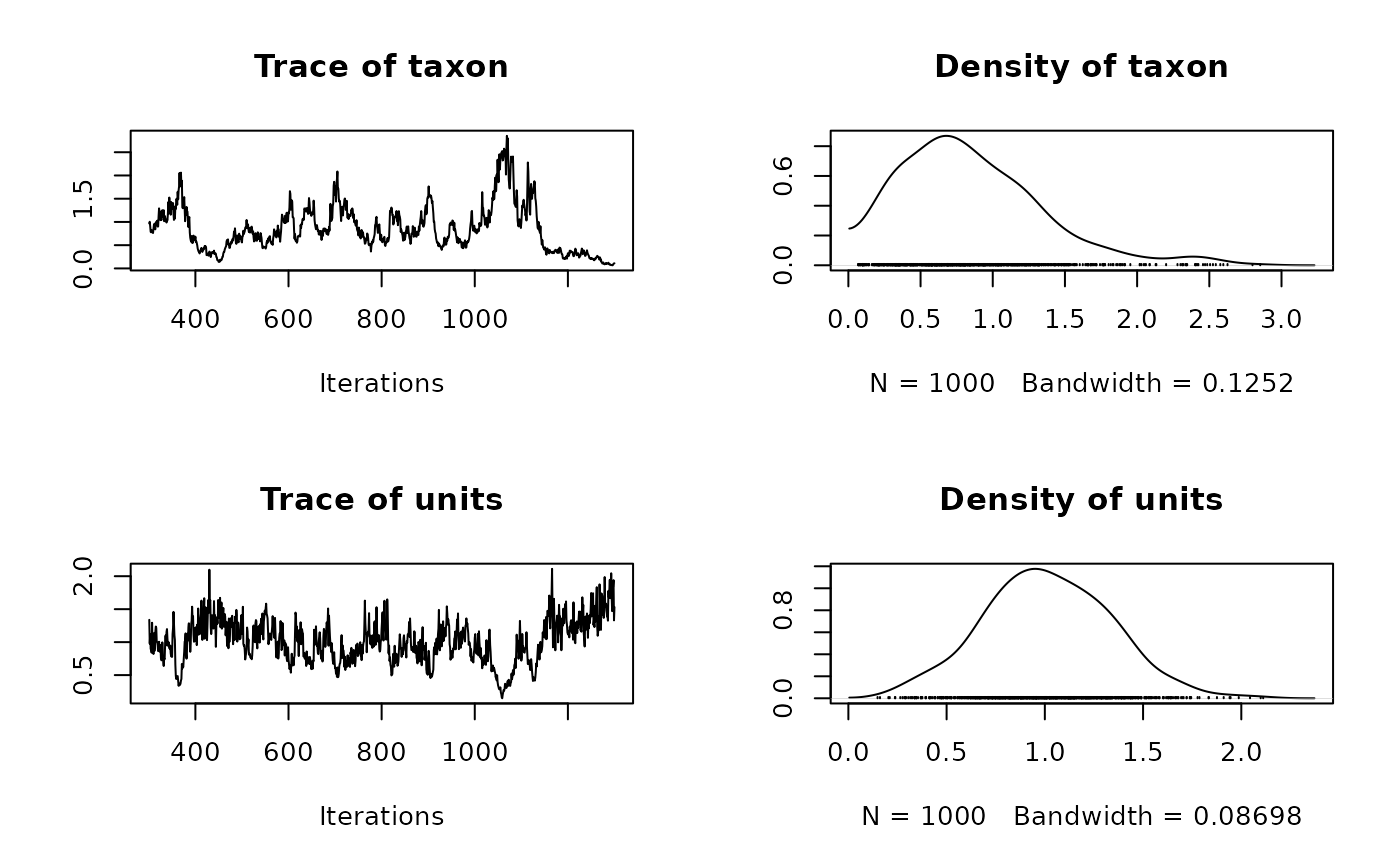
model2<-MCMCglmm(phenotype~1, random=~taxon, ginverse=list(taxon=Ainv),
 data=test.data, prior=prior, verbose=FALSE, nitt=1300, burnin=300, thin=1)

plot(model2$VCV)